Time indexes and temporal aggregation

This tutorial starts with something very fundamental that people often do not think about for a long time: The choice of the time increment. This part is independent from solph and very suitable for beginners. The last steps are presenting experimental features of solph, namely time series aggregation and pathway planning. These can be considered advanced usage. The full tutorial consists of the following:

• Step 1: Sampling of high resolution input data

• Step 2: Upfront investment using different time resolutions

• Step 3: Upfront investment using time series aggregation

• Step 4: Pathway planning using time series aggregation

Step 1: Sampling of high resolution input data

Temporal and spatial resolution are often connected. If you average over multiple locations, volatililty in the data is reduced, reducing the effect of temporal aggregation. We take a detatched single family home with just one inhabitant as our basis, because a significant influence of the aggregation is expected here. Further, we use real-world data as synthetic data might feature repetitive features, putting a bias to the aggreagtion that is planned later.

We use building 27 plus the south-facing PV from the one-minute resolution dataset described of the Dataset on electrical single-family house and heat pump load profiles in Germany, which is also available at doi: 10.5281/zenodo.5642902. The data is licensed from M. Schlemminger, T. Ohrdes, E. Schneider, and M. Knoop under Creative Commons Attribution 4.0 International License.

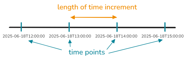
But first, let us go through some basics about the time index. As mentioned in Energy System, we use N+1 points in time to define N time intervals. At the first glance, this might seem to add extra complication, but being explicit and clear helps formulating models that are precise, comprehensible, and physically correct. The function solph.create_time_index() takes the number of time intervals as a input, so you can take a shortcut here:

>>> from oemof import solph
>>> es = solph.EnergySystem(
...    timeindex=solph.create_time_index(2025, interval=0.5, number=2)
... )
>>> print(list(es.timeindex))
[Timestamp('2025-01-01 00:00:00'), Timestamp('2025-01-01 00:30:00'), Timestamp('2025-01-01 01:00:00')]

>>> print(list(es.timeincrement))
[0.5, 0.5]

It should be mentioned that the exact time stamp helps with data processing but is not relevant for the optimisation. Thus, you can also give a number of ascending values. The time increment then is the difference between those. Except for the time index, the following energy system will produce exactly the same results.

>>> from oemof import solph
>>> es = solph.EnergySystem(timeindex=[2, 2.5, 3])
>>> print(es.timeindex)
[2, 2.5, 3]
>>> print(list(es.timeincrement))
[0.5, 0.5]

Now, that we know how time steps are defined, let us look at a good choice for the time intervals. Often, time steps are chosen to have the same length. This is advantegous as they make the model easy to comprehend, as you can convert between counting indexes and time by multiplying a constant. This particularly simplifies formulations of constraints to the extend that some uncommon use cases of solph are currently bound to fixed intervals. Let us go through this based on our input data.

if __name__ == "__main__":
    import matplotlib.pyplot as plt

    my_df = prepare_input_data()

    resolutions = [
        "1 min",
        "15 min",
        "1 h",
        "3 h",
    ]

    fig0, ax0 = plt.subplots(figsize=(4, 2), tight_layout=True)
    fig1, ax1 = plt.subplots(figsize=(4, 2), tight_layout=True)

    for resolution in resolutions:
        time_series = 15.4 * my_df["PV (kW/kWp)"].resample(resolution).mean()

        time_series = time_series[
            datetime.datetime(
                2019, 11, 3, 0, tzinfo=datetime.timezone.utc
            ) : datetime.datetime(2019, 11, 4, 0, tzinfo=datetime.timezone.utc)
        ]
        hour_axis = np.linspace(0, 24, num=len(time_series))
        ax0.step(
            x=hour_axis,
            y=time_series,
            label=resolution,
            where="post",
        )
        ax1.step(
            x=hour_axis,
            y=sorted(time_series)[::-1],
            label=resolution,
            where="post",
        )

    ax0.set_xlim(5.9, 18.1)
    ax0.set_xlabel("Time (UTC)")
    ax0.set_ylabel("Power (kW)")
    ax0.legend()
    ax0.grid()
    fig0.savefig("2019-11-3_PV-timeseries.svg")

    ax1.grid()
    ax1.set_xlim(-0.1, 12.1)
    ax1.set_xlabel("Duration (h)")
    ax1.set_ylabel("Power (kW)")
    ax1.set_yscale("log")
    fig1.savefig("2019-11-3_PV-duration.svg")

    plt.show()

The script reads in the data, defines desired resolutions, and then creates two figures, one for a time series plot, one for a duration curve. In the loop, it resamples the data to the set resolution and produces the step graphs for the two types of plots. An example output is included in the following:

Of course, one day is not representative, but it is clearly visible that even the resolution of 15-minutes cannot preserve the dynamics of the data. Further, it should be noted that averaging the power values reduces the peaks, while the total energy is preserved. Thus, the lower resolutions systematically overestimate low loads. Also note that we cut of the night from the graph, because in the corresponding hours the PV data of course shows a flat zero. So, what if we also just drop the nights from our data? This is done by the following function, which just hardcodes the day to be between 5 am and 9 pm. There are two nocturnal time steps of four hours each, which extend from 9pm to 1 am and from 1 am to 5 am. This is a conservative assumption, that should work all year long, but already reduces the number of time steps by 25 %.

def reshape_unevenly(data):
    def to_bucket(ts: pd.Timestamp) -> pd.Timestamp:
        h = ts.hour
        d = ts.normalize()
        if 5 <= h <= 20:
            return ts
        if h in (21, 22, 23):
            return d + pd.Timedelta(hours=21)
        if h in (0,):
            return (d - pd.Timedelta(days=1)) + pd.Timedelta(hours=21)
        # h in (1, 2, 3, 4, 5)
        return d + pd.Timedelta(hours=1)

    buckets = data.index.map(to_bucket)
    buckets = buckets.where(buckets >= data.index[0], data.index[0])

    data_mean = data.groupby(buckets).mean().sort_index()
    data_mean.index.name = "timestamp"

    return data_mean

Now, how will an optimisation problem react to this reduction? Let us have a look!

Step 2: Setting up the Energy System Model

Setting up energy systems has already been discussed in the other tutorials. Thus, we only stay on the surface here. The model describes a (potentially all-electric) single-family home. There are demands that cannot be optimised, in contrast to the EV tutorial, here we also consider the wall box a fixed demand.

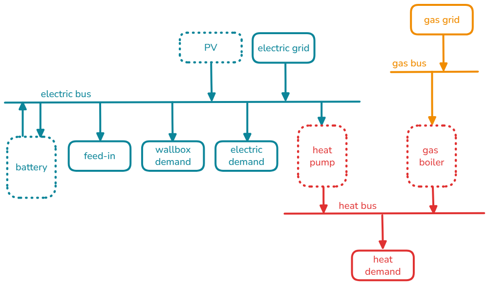
The energy system allows investments into battery (GenericStorage), pv (Flow out of a Source), as well as a heat pump and a gas boiler (boths Flow s out of Converter s). For reference, you can have a look at the full code until here:

timeindex_1_segmentation.py

Click to display the code

# -*- coding: utf-8 -*-

"""
SPDX-FileCopyrightText: Uwe Krien
SPDX-FileCopyrightText: Patrik Schönfeldt
SPDX-FileCopyrightText: DLR e.V.

SPDX-License-Identifier: MIT
"""

import logging
import warnings
from collections import namedtuple
from datetime import datetime
from pathlib import Path

import pandas as pd
from input_data import discounted_average_price
from input_data import energy_prices
from input_data import get_parameter
from input_data import investment_costs
from input_data import prepare_input_data
from oemof.tools import debugging
from oemof.tools import logger
from oemof.tools.economics import annuity

from oemof import solph

warnings.filterwarnings(
    "ignore", category=debugging.ExperimentalFeatureWarning
)
logger.define_logging()


def calculate_fix_cost(value):
    return value / 20


# %%[reshape_unevenly]
def reshape_unevenly(data):
    def to_bucket(ts: pd.Timestamp) -> pd.Timestamp:
        h = ts.hour
        d = ts.normalize()
        if 5 <= h <= 20:
            return ts
        if h in (21, 22, 23):
            return d + pd.Timedelta(hours=21)
        if h in (0,):
            return (d - pd.Timedelta(days=1)) + pd.Timedelta(hours=21)
        # h in (1, 2, 3, 4, 5)
        return d + pd.Timedelta(hours=1)

    buckets = data.index.map(to_bucket)
    buckets = buckets.where(buckets >= data.index[0], data.index[0])

    data_mean = data.groupby(buckets).mean().sort_index()
    data_mean.index.name = "timestamp"

    return data_mean

# %%[prepare_technical_data]
def prepare_technical_data(minutes, url, port):
    data = namedtuple("data", "even uneven")
    data_table = (
        prepare_input_data(proxy_url=url, proxy_port=port)
        .resample(f"{minutes} min")
        .mean()
    )
    df_un = reshape_unevenly(data_table)
    return data(even=data_table, uneven=df_un)


def prepare_cost_data():
    pass


def populate_and_solve_energy_system(
    es: solph.EnergySystem,
    time_series: dict[str, list] | dict[str, pd.DataFrame],
    investments: dict[str, solph.Investment],
    variable_costs: dict | pd.DataFrame,
    discount_rate=0.02,
):

    parameter = get_parameter()

    bus_el = solph.Bus(label="electricity")
    bus_heat = solph.Bus(label="heat")
    bus_gas = solph.Bus(label="gas")
    es.add(bus_el, bus_heat, bus_gas)

    es.add(
        solph.components.Source(
            label="PV",
            outputs={
                bus_el: solph.Flow(
                    fix=time_series["PV (kW/kWp)"],
                    nominal_capacity=investments["pv"],
                )
            },
        )
    )

    es.add(
        solph.components.GenericStorage(
            label="Battery",
            inputs={bus_el: solph.Flow()},
            outputs={bus_el: solph.Flow()},
            nominal_capacity=investments["battery"],  # kWh
            loss_rate=parameter["loss_rate_battery"],
            inflow_conversion_factor=parameter["charge_efficiency_battery"],
            outflow_conversion_factor=parameter[
                "discharge_efficiency_battery"
            ],
        )
    )

    es.add(
        solph.components.Sink(
            label="Electricity demand",
            inputs={
                bus_el: solph.Flow(
                    fix=time_series["electricity demand (kW)"],
                    nominal_capacity=1.0,
                )
            },
        )
    )

    wallbox_sink = solph.components.Sink(
        label="Electric Vehicle",
        inputs={
            bus_el: solph.Flow(
                fix=time_series["Electricity for Car Charging_HH1"],
                nominal_capacity=1.0,
            )
        },
    )
    es.add(wallbox_sink)

    hp = solph.components.Converter(
        label="Heat pump",
        inputs={bus_el: solph.Flow()},
        outputs={
            bus_heat: solph.Flow(nominal_capacity=investments["heat pump"])
        },
        conversion_factors={bus_heat: time_series["cop"]},
    )
    es.add(hp)

    gas_boiler = solph.components.Converter(
        label="Gas Boiler",
        inputs={bus_gas: solph.Flow()},
        outputs={
            bus_heat: solph.Flow(nominal_capacity=investments["gas boiler"])
        },
        conversion_factors={bus_heat: parameter["efficiency_boiler"]},
    )
    es.add(gas_boiler)

    heat_sink = solph.components.Sink(
        label="Heat demand",
        inputs={
            bus_heat: solph.Flow(
                fix=time_series["heat demand (kW)"],
                nominal_capacity=1.0,
            )
        },
    )
    es.add(heat_sink)

    grid_import = solph.components.Source(
        label="Grid import",
        outputs={
            bus_el: solph.Flow(
                variable_costs=variable_costs["electricity_prices [Eur/kWh]"]
            )
        },
    )
    es.add(grid_import)

    feed_in = solph.components.Sink(
        label="Grid Feed-in",
        inputs={
            bus_el: solph.Flow(
                variable_costs=variable_costs["pv_feed_in [Eur/kWh]"]
            )
        },
    )
    es.add(feed_in)

    gas_import = solph.components.Source(
        label="Gas import",
        outputs={
            bus_gas: solph.Flow(
                variable_costs=variable_costs["gas_prices [Eur/kWh]"]
            )
        },
    )
    es.add(gas_import)

    logging.info("Creating Model...")
    m = solph.Model(es, discount_rate=discount_rate)
    logging.info("Solving Model...")

    results = m.solve(solver="cbc", solve_kwargs={"tee": False})

    return results


def solve_model(data, parameter, year=2025, es=None):
    if es is None:
        es = solph.EnergySystem(timeindex=data.index)

    var_cost = discounted_average_price(
        price_series=energy_prices(),
        observation_period=parameter["n"],
        interest_rate=parameter["r"],
        year_of_investment=year,
    )
    investments = create_investment_objects(
        n=parameter["n"],
        r=parameter["r"],
        year=year,
    )
    results = populate_and_solve_energy_system(
        es=es,
        time_series=data,
        investments=investments,
        variable_costs=var_cost,
    )

    return results


def create_investment_objects(n, r, year):
    invest_cost = investment_costs().loc[year]

    # Create Investment objects from cost data
    investments = {}
    for key in ["gas boiler", "heat pump", "battery", "pv"]:
        try:
            epc = annuity(
                invest_cost[(key, "specific_costs [Eur/kW]")],
                n=n,
                wacc=r,
            )
            maximum = invest_cost[(key, "maximum [kW]")]
        except KeyError:
            epc = annuity(
                invest_cost[(key, "specific_costs [Eur/kWh]")],
                n=n,
                wacc=r,
            )
            maximum = invest_cost[(key, "maximum [kWh]")]
        fix_cost = annuity(
            invest_cost[(key, "fixed_costs [Eur]")],
            n=n,
            wacc=r,
        )

        investments[key] = solph.Investment(
            ep_costs=epc,
            offset=fix_cost,
            maximum=maximum,
            lifetime=20,
            nonconvex=bool(fix_cost > 0),  # need to cast to avoid np.bool
        )
    return investments


def process_results(results):
    key_results = results["invest"].rename(
        columns={
            c: c[0].label
            for c in results["invest"].columns
            if isinstance(c, tuple)
        },
    )
    key_results["objective"] = results["objective"]
    return key_results


def optimise_investment(year, interval, result_path):
    result_file = f"time_series_even_uneven_{year}_{interval}min.csv"
    result_fn = Path(result_path, result_file)

    if not result_fn.is_file():
        logging.info(f"Start with {year} - {interval}")
        # Create empty file
        with open(result_fn, "w")  as file:
            file.write(f"Start with {year} - {interval}")
        my_data = prepare_technical_data(interval, None, None)

        logging.info("Start with even....")
        start = datetime.now()
        results_even = solve_model(my_data.even, get_parameter(), year=year)
        key_results_even = process_results(results_even)
        key_results_even["short_interval"] = interval
        key_results_even["year_of_investment"] = year
        time_even = datetime.now() - start
        key_results_even["time"] = time_even.seconds

        logging.info("Start with uneven....")
        start = datetime.now()
        results_uneven = solve_model(
            my_data.uneven, get_parameter(), year=year
        )
        key_results_uneven = process_results(results_uneven)
        time_uneven = datetime.now() - start
        key_results_uneven["time"] = time_uneven.seconds

        logging.info("Create joined results.")
        results = (
            pd.concat(
                [key_results_uneven, key_results_even],
                keys=["uneven", "even"],
            )
            .droplevel(1)
            .T
        )
        results.to_csv(result_fn)

        # compare_results(results_even, results_uneven)
        print()
        print("*** Investment ***")
        print("even\n", key_results_even.iloc[0])
        print("uneven\n", key_results_uneven.iloc[0])
        print()
        print("*** Times ****")
        print("even", time_even)
        print("uneven", time_uneven)


def read_result_files(year, interval, result_path):
    result_file = f"time_series_even_uneven_{year}_{interval}min.csv"
    temp = pd.read_csv(Path(result_path, result_file), index_col=[0])
    temp = pd.concat([temp], keys=[interval], axis=1)
    return pd.concat([temp], keys=[year], axis=1)


if __name__ == "__main__":
    my_result_path = Path(Path.home(), ".oemof", "tutorial", "time_series")
    my_result_path.mkdir(parents=True, exist_ok=True)
    intervals = [60, 30, 15, 10, 5, 1]
    years = [2025, 2035, 2045]

    for my_year in years:
        for my_interval in intervals:
            optimise_investment(my_year, my_interval, my_result_path)

    df = pd.DataFrame()
    for my_year in years:
        for my_interval in intervals:
            df = pd.concat(
                [df, read_result_files(my_year, my_interval, my_result_path)],
                axis=1,
            )

    df.sort_index(axis=1).to_csv(Path(my_result_path, "results_all.csv"))

Step 3: Optimization using time series aggregation

In this section, we introduce time series aggregation with tsam - time series aggregation module.

At the time of writing, the TSAM integration in oemof.solph is implemented via the multi-period (pathway planning) interface. For Step 3, we use exactly one investment period. This means that investment decisions are still made once for the whole horizon (as in the standard upfront-investment approach from Step 2), but the operational time series are replaced by an aggregated representation.

Please note that this feature is still experimental and may therefore contain bugs.

We use the same input data and energy system setup as in Step 1 and Step 2.

Concept: clustering to typical periods

The basic idea of time series aggregation for energy system design is to replace a long time series (e.g. one year of hourly data) by a small set of representative periods (often called typical periods). The optimisation problem is then solved only for these typical periods, while the objective function accounts for how often each typical period occurs in the original time set.

Example: A full year (365 days) can be clustered into 10 typical periods of length 24 hours. In other words, the year is represented by 10 typical days (A, B, C, ...) plus an order that maps each original day to one of these typical days in th year:

(A, A, B, A, A, C, A ..., C)

Variable flows in the objective function are weighted according to the frequency of their corresponding typical periods in the original time set.

If a storage is included, the typical periods must be linked to represent storage carry-over between periods. For this, we use an approach introduced by Kotzur et al. by splitting the storage state into two parts:

• intra storage level: the change of storage level within a typical period

• inter storage level: the storage level in between two periodd in the original sequence of periods

The total storage level is represented as a superposition of both. For details, see Time series aggregation for energy system design: Modeling seasonal storage.

Effect on the optimisation model

To explain on a high level the influence on our optimization model, we use the 10 typical days example (A, B, C, ...):

Without storage, the operational part of the model is reduced because only the flows for the typical days are optimised (10 × 24 hours), instead of all 365 days.

With storage, the model still optimises the flows for the typical periods. In addition, the intra storage level is optimised for each representative period (10 × 24 hours). In our example with 24-hour periods, the original time set is split into 365 periods. Therefore the inter-period storage level occurs 365 times (one value per original day). Overall, this typically leads to a significant reduction in runtime.,

If you add constraints with binary variables, an important modelling question is which time grid these binaries should use when using TSAM. For a first insight, see Operational Optimization of Seasonal Ice-Storage Systems with Time-Series Aggregation.

Clustering the input time series with TSAM

To cluster input time series with TSAM, you need to define:

• noTypicalPeriods: the number of typical periods (e.g. 10 typical days)

• hoursPerPeriod: the length of each period in hours (e.g. 24 for typical days)

• clusterMethod: the clustering algorithm

These parameter names follow TSAM’s terminology. In this tutorial we use hourly data. Non-hourly resolutions might be possible to solve, but isn’t tested in detail.

The influence of different aggregation methods is discussed in Impact of different time series aggregation methods on optimal energy system design.

The clustering step can then be implemented as follows:

    # --- TSAM clustering ---
    aggregation = tsam.TimeSeriesAggregation(
        timeSeries=data.iloc[:8760],
        noTypicalPeriods=typical_periods,
        hoursPerPeriod=hours_per_period,
        clusterMethod="k_means",
        sortValues=False,
        rescaleClusterPeriods=False,
    )
    aggregation.createTypicalPeriods()

Building the energy system with an aggregated time index

Compared to the standard approach, setting up the EnergySystem differs slightly. In addition to the aggregated timeindex, you need to provide:

• timesteps_per_period: number of time steps per typical period

• order: mapping from original periods to typical periods

This is shown in the following snippet:

    tindex_agg = pd.date_range(
        "2022-01-01",
        periods=len(aggregation.clusterPeriodIdx) * hours_per_period,
        freq="h",
    )

    es = solph.EnergySystem(
        timeindex=tindex_agg,
        timeincrement=[1] * len(tindex_agg),
        periods=[tindex_agg],
        tsa_parameters=[
            {
                "timesteps_per_period": aggregation.hoursPerPeriod,
                "order": aggregation.clusterOrder,
                "timeindex": aggregation.timeIndex,
            }
        ],
        infer_last_interval=False,
    )

Post-processing and sensitivity to aggregation choices

In post-processing, the optimised flows and storage levels are disaggregated back to the original time grid. This means you can process and plot results in the same way as in the non-aggregated examples.

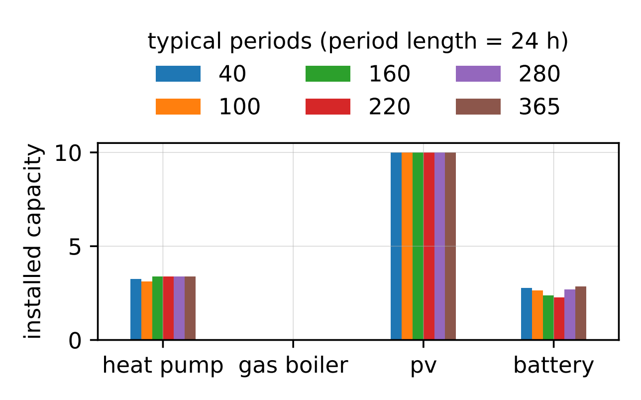
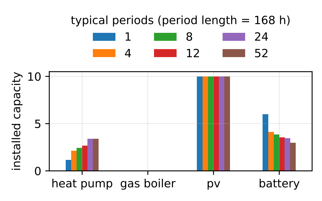
However, the choice of aggregation parameters (number and length of typical periods) can have a strong influence on the results. To illustrate this, we run the optimisation for different numbers of typical periods, using typical period lengths of 24 hours and 168 hours:

The complete code for this step can be found at:

timeindex_2_typical_periods.py

Click to display the code

import warnings
from datetime import datetime

import pandas as pd
import tsam.timeseriesaggregation as tsam
from input_data import discounted_average_price
from input_data import energy_prices
from input_data import get_parameter
from input_data import investment_costs
from input_data import prepare_input_data
from matplotlib import pyplot as plt
from oemof.tools import debugging
from oemof.tools import logger
from timeindex_1_segmentation import populate_and_solve_energy_system

from oemof import solph

warnings.filterwarnings(
    "ignore", category=debugging.ExperimentalFeatureWarning
)
logger.define_logging()

# -----------------------------
# Global inputs (once)
# -----------------------------
data = prepare_input_data()
data = data.resample("1 h").mean()

year = 2025
parameter = get_parameter()

variable_costs = discounted_average_price(
    price_series=energy_prices(),
    observation_period=parameter["n"],
    interest_rate=parameter["r"],
    year_of_investment=year,
)


def create_investment_objects_multi_period(year_of_invest):
    invest_cost = investment_costs().loc[year_of_invest]

    # Create Investment objects from cost data
    investments = {}
    for key in ["gas boiler", "heat pump", "battery", "pv"]:
        try:
            epc = invest_cost[(key, "specific_costs [Eur/kW]")]

            maximum = invest_cost[(key, "maximum [kW]")]
        except KeyError:
            epc = invest_cost[(key, "specific_costs [Eur/kWh]")]
            maximum = invest_cost[(key, "maximum [kWh]")]

        fix_cost = invest_cost[(key, "fixed_costs [Eur]")]

        investments[key] = solph.Investment(
            ep_costs=epc,
            offset=fix_cost,
            maximum=maximum,
            lifetime=20,
            nonconvex=True,
        )
    return investments


investment_objects = create_investment_objects_multi_period(
    year_of_invest=year,
)


def run_for_typical_periods(
    typical_periods: int, hours_per_period: int = 24
) -> pd.Series:
    """
    Run the full TSAM aggregation + oemof optimization for one typical_periods
    value.
    Returns installed capacities as a Series (PV kW, Battery kWh, HP kW, Gas
    boiler kW).
    """
    # %%[tsam_aggregation_start]
    # --- TSAM clustering ---
    aggregation = tsam.TimeSeriesAggregation(
        timeSeries=data.iloc[:8760],
        noTypicalPeriods=typical_periods,
        hoursPerPeriod=hours_per_period,
        clusterMethod="k_means",
        sortValues=False,
        rescaleClusterPeriods=False,
    )
    aggregation.createTypicalPeriods()
    # %%[tsam_aggregation_end]
    time_series = {
        "cop": aggregation.typicalPeriods["cop"],
        "electricity demand (kW)": aggregation.typicalPeriods[
            "electricity demand (kW)"
        ],
        "heat demand (kW)": aggregation.typicalPeriods["heat demand (kW)"],
        "PV (kW/kWp)": aggregation.typicalPeriods["PV (kW/kWp)"],
        "Electricity for Car Charging_HH1": aggregation.typicalPeriods[
            "Electricity for Car Charging_HH1"
        ],
    }
    # %%[ti_index_and_energy_system_start]
    tindex_agg = pd.date_range(
        "2022-01-01",
        periods=len(aggregation.clusterPeriodIdx) * hours_per_period,
        freq="h",
    )

    es = solph.EnergySystem(
        timeindex=tindex_agg,
        timeincrement=[1] * len(tindex_agg),
        periods=[tindex_agg],
        tsa_parameters=[
            {
                "timesteps_per_period": aggregation.hoursPerPeriod,
                "order": aggregation.clusterOrder,
                "timeindex": aggregation.timeIndex,
            }
        ],
        infer_last_interval=False,
    )
    # %%[ti_index_and_energy_system_end]
    results = populate_and_solve_energy_system(
        es=es,
        time_series=time_series,
        investments=investment_objects,
        variable_costs=variable_costs,
    )

    # The keys actually contain the Nodes and not strings,
    # but as a Node is equal to its string, the following works.
    pv_invest_kw = results["invest"][("PV", "electricity")][0]
    storage_invest_kwh = results["invest"]["Battery"][0]
    hp_invest_kw = results["invest"][("Heat pump", "heat")][0]
    gas_boiler_invest_kw = results["invest"][("Gas Boiler", "heat")][0]

    return pd.Series(
        {
            "PV": pv_invest_kw,
            "Battery": storage_invest_kwh,
            "HP": hp_invest_kw,
            "Gas boiler": gas_boiler_invest_kw,
        },
        name=f"{typical_periods}",
    )


# -----------------------------
# Config for both aggregations
# -----------------------------
configs = [
    {"hours_per_period": 24, "typical_periods": [40, 100, 160, 220, 280, 365]},
    {"hours_per_period": 24 * 7, "typical_periods": [1, 4, 8, 12, 24, 52]},
]

caps_by_hpp = {}  # store results per hours_per_period


# -----------------------------
# Run for multiple typical periods AND multiple hours_per_period
# -----------------------------
computation_time = {}
for cfg in configs:
    hpp = cfg["hours_per_period"]
    tp_list = cfg["typical_periods"]

    all_caps = []
    for tp in tp_list:
        start = datetime.now()
        all_caps.append(run_for_typical_periods(tp, hours_per_period=hpp))
        computation_time[hpp, tp] = datetime.now() - start

    capas_df = pd.concat(all_caps, axis=1)
    capas_df.columns = [int(c) for c in capas_df.columns]
    caps_by_hpp[hpp] = capas_df

print(pd.Series(computation_time))


# -----------------------------
# Plotting helper
# -----------------------------
def plot_caps(
    caps_df: pd.DataFrame, hours_per_period: int, filename_prefix: str
):
    fig, ax = plt.subplots(figsize=(4, 2.5), tight_layout=True)

    caps_df.plot(kind="bar", ax=ax)

    ax.set_ylabel("Installed capacity")  # explain mixed units in caption
    ax.set_xlabel(None)
    ax.grid(True, linewidth=0.3, alpha=0.6)

    # Put the period duration "cleverly" into the legend title
    ax.legend(
        title=f"Typical periods (period length = {hours_per_period} h)",
        ncol=3,
        frameon=False,
        loc="lower center",
        bbox_to_anchor=(0.5, 1.02),
    )

    ax.tick_params(axis="x", rotation=0)

    fig.savefig(f"{filename_prefix}.eps")
    fig.savefig(f"{filename_prefix}.pdf")

    return fig, ax


# -----------------------------
# Create TWO plots
# -----------------------------
plot_caps(
    caps_by_hpp[24],
    hours_per_period=24,
    filename_prefix="investments_bar_tp_daily",
)

plot_caps(
    caps_by_hpp[24 * 7],
    hours_per_period=24 * 7,
    filename_prefix="investments_bar_tp_weekly",
)

plt.show()

Step 4: Pathway planning using time series aggregation

In this section, we introduce pathway planning. Please note that this feature is still experimental and may therefore contain bugs (known issues discovered while preparing this tutorial will be discussed).

Pathway planning differs from the previous examples in an important way: investment variables become time-dependent. In the previous cases, all investment decisions were made once for the entire optimization horizon. In pathway planning, investments may change at predefined points in time. These points represent the years or periods in which new investments can be made (or existing ones can be expanded).

Typically, investment decisions do not need to change as frequently as the operational time steps of the model. For example, while the model may run on hourly resolution, investment decisions might only be updated every five years. Therefore, you need to define two kinds of time indices:

1. A “normal” time index for the operational resolution (discussed earlier)

2. A set of investment times/periods (times when new capacity can be installed)

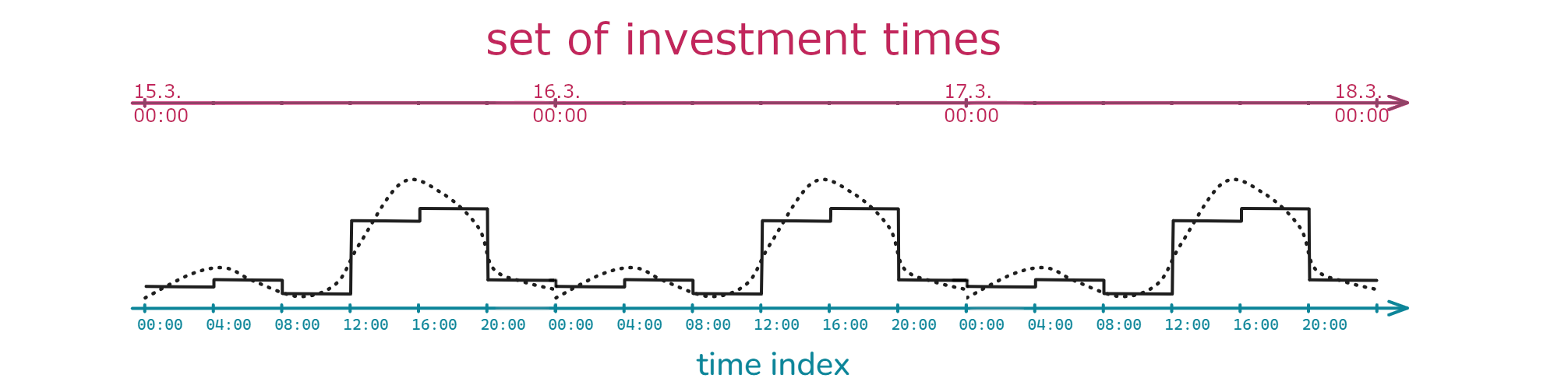
Although pathway planning is theoretically compatible with all previously discussed ways of defining time indices, in the current version of oemof.solph you must use time series aggregation together with pathway planning. (We aim to remove this restriction in future versions.)

Starting from your original one-year dataset (and assuming that demand and generation patterns do not change significantly between years), you create an aggregated time index in the same way as in Step 3.

typical_periods = 100
hours_per_period = 24

start = datetime.now()

aggregation = tsam.TimeSeriesAggregation(
    timeSeries=data.iloc[:8760],
    noTypicalPeriods=typical_periods,
    hoursPerPeriod=hours_per_period,
    clusterMethod="k_means",
    sortValues=False,
    rescaleClusterPeriods=False,
)
aggregation.createTypicalPeriods()

# create a time index for the aggregated time series
tindex_agg = pd.date_range(
    "2025-01-01", periods=typical_periods * hours_per_period, freq="h"
)

# ------------ create timeindex etc. for multiperiod --------------------------

To implement pathway planning in solph, three additional steps are required:

1. Build one continuous operational time index covering the entire optimization horizon.

2. Create a list of time indices, one for each investment period.

3. Create a dictionary of TSAM parameters, also one entry per investment period.

Suppose you want to allow investment changes every five years, e.g. in [2025, 2030, 2035, 2040, 2045]. To reduce runtime, each 5‑year period will be represented by one aggregated year.

Currently, oemof.solph does not support “skipping” years directly. Therefore, you must as a work around define investment years as a continuous sequence, e.g.:

[2025, 2026, 2027, 2028, 2029]

These then can be mapped to your intenden resolution of five years. This will require some preprocessing in cost data etc., which will be explained further down.

You can then perform the three steps described above:

# create a time index for the whole model
# Create a list of shifted copies of the original index,
# one per investment year
base_year = years[0]
shifted = [tindex_agg + pd.DateOffset(years=(y - base_year)) for y in years]

# Concatenate them into one DatetimeIndex
tindex_agg_full = shifted[0]
for s in shifted[1:]:
    tindex_agg_full = tindex_agg_full.append(s)

print("------- Time Index of Multi-Period Model --------")
print("time index: ", tindex_agg_full)
print("-------------------------------------------------")

# create the list of investment periods for the model
investment_periods = [
    tindex_agg + pd.DateOffset(years=i) for i in range(len(years))
]


print("------- Priods of Multi-Period Model --------")
print("Investment periods: ", investment_periods)
print("---------------------------------------------")

# create parameters for time series aggregation in oemof-solph
# with one dict per year
tsa_parameters = [
    {
        "timesteps_per_period": aggregation.hoursPerPeriod,
        "order": aggregation.clusterOrder,
        "timeindex": tindex_agg + pd.DateOffset(years=i),
    }
    for i in range(len(years))
]

Next, you can build your energy system:

es = solph.EnergySystem(
    timeindex=tindex_agg_full,
    timeincrement=timeincrement,
    periods=investment_periods,
    tsa_parameters=tsa_parameters,
    infer_last_interval=False,
    use_remaining_value=True,
)

Now the hardest part is done!

From here, you can construct your system exactly as in previous examples. However, keep in mind:

• All operational time series must span the entire optimization horizon

• Their index/length must match the combined time index you created earlier

Since we assume that demand and production profiles remain constant across years, we can simply repeat the original one-year dataset over the length of the horizon:

timeincrement = [1] * (len(tindex_agg_full))

time_series = {
    "cop": pd.concat(
        [aggregation.typicalPeriods["cop"]] * len(years),
        ignore_index=True,
    ),
    "electricity demand (kW)": pd.concat(
        [aggregation.typicalPeriods["electricity demand (kW)"]] * len(years),
        ignore_index=True,
    ),
    "heat demand (kW)": pd.concat(
        [aggregation.typicalPeriods["heat demand (kW)"]] * len(years),
        ignore_index=True,
    ),
    "PV (kW/kWp)": pd.concat(
        [aggregation.typicalPeriods["PV (kW/kWp)"]] * len(years),
        ignore_index=True,
    ),
    "Electricity for Car Charging_HH1": pd.concat(
        [aggregation.typicalPeriods["Electricity for Car Charging_HH1"]]
        * len(years),
        ignore_index=True,
    ),
}

Although the model internally treats each period as one year, investment decisions actually represent five-year steps (as discussedabove). To maintain the correct ratio of investment costs to variable costs, we scale the lifetime and investment costs by the length of the investment period.

Example: A battery has a real lifetime of 10 years. Since one model “year” represents 5 real years:

• Effective lifetime in the model: 10 / 5 = 2

• Investment costs and offsets must also be divided by 5

This ensures that discounting and cost comparisons remain realistic.

investments = {
    "pv": solph.Investment(
        ep_costs=investment_costs[("pv", "specific_costs [Eur/kW]")] / 5,
        lifetime=4,
        nonconvex=True,
        offset=investment_costs[("pv", "fixed_costs [Eur]")] / 5,
        maximum=10,
        overall_maximum=10,
    ),
    "battery": solph.Investment(
        ep_costs=investment_costs[("battery", "specific_costs [Eur/kWh]")] / 5,
        lifetime=2,
    ),
    "heat pump": solph.Investment(
        ep_costs=investment_costs[("heat pump", "specific_costs [Eur/kW]")]
        / 5,
        lifetime=4,
        nonconvex=True,
        offset=investment_costs[("heat pump", "fixed_costs [Eur]")] / 5,
        maximum=10,
        overall_maximum=10,
    ),
    "gas boiler": solph.Investment(
        ep_costs=investment_costs[("gas boiler", "specific_costs [Eur/kW]")]
        / 5,
        lifetime=4,
        fixed_costs=investment_costs[("gas boiler", "fixed_costs [Eur]")] / 5,
        existing=3.5,  # existing cannot be combined with nonconvex
        age=2,
    ),
}

# ------------------ create energy system -------------------------------------

Finally, adjust the discount rate to reflect that each model period represents five real years. This ensures that net‑present‑value calculations are consistent with your investment period length:

def discount_rate_adjusted(discount_rate, investment_period_length_in_years):
    return (1 + discount_rate) ** investment_period_length_in_years - 1

Now you can solve the model and plot the results:

The complete code for this step can be found at:

timeindex_3_pathway_planning.py

Click to display the code

# -*- coding: utf-8 -*-
import warnings
from datetime import datetime

import matplotlib.pyplot as plt
import pandas as pd
import tsam.timeseriesaggregation as tsam
from input_data import energy_prices
from input_data import investment_costs
from input_data import prepare_input_data
from oemof.tools import debugging
from oemof.tools import logger
from timeindex_1_segmentation import populate_and_solve_energy_system

from oemof import solph
from oemof.solph import Results


# ---------------- some helper functions --------------------------------------
def lifetime_adjusted(lifetime, investment_period_length_in_years):
    return int(lifetime / investment_period_length_in_years)


# %% [discount]
def discount_rate_adjusted(discount_rate, investment_period_length_in_years):
    return (1 + discount_rate) ** investment_period_length_in_years - 1


# %% [expand]
def expand_energy_prices(tidx_agg_full, e_prices):
    years_in_index = sorted(set(tidx_agg_full.year))
    years_available = set(e_prices.index)

    # Strict check: all years in the index must be present in the table
    missing = [y for y in years_in_index if y not in years_available]
    if missing:
        raise KeyError(f"Missing prices for years in index: {missing}")

    # Build a year->price lookup and vectorized map
    df = pd.DataFrame()
    for col in e_prices.columns:
        year_prices = e_prices[col]
        df[col] = pd.Series(
            pd.Series(tidx_agg_full.year).map(year_prices).values,
            index=tidx_agg_full,
            name=col,
        )
    return df


# -----------------------------------------------------------------------------
warnings.filterwarnings(
    "ignore", category=debugging.ExperimentalFeatureWarning
)
logger.define_logging()

# ---------- read cost data ---------------------------------------------------

investment_costs = investment_costs()
prices = energy_prices()

# Note:
# originally the data provided is for investment periods of 5 years each
# so years = [2025, 2030, 2035, 2040, 2045]
# this was causing a bug in the mulit period calculation of the fixed_costs in
# the INVESTFLOWS, therefore years is set to [2025, 2026, 2027, 2028, 2029] in
# this example this will be changed, when the bug is fixed

# list with years in which investment is possible
years = [2025, 2026, 2027, 2028, 2029]

investment_costs_new = investment_costs.loc[[2025, 2030, 2035, 2040, 2045]]
investment_costs_new.index = years
investment_costs = investment_costs_new

prices_new = prices.loc[[2025, 2030, 2035, 2040, 2045]]
prices_new.index = years
prices = prices_new

# ---------- read time series data and resample--------------------------------

data = prepare_input_data()

data = data.resample("1 h").mean()
print(data)

# -------------- Clustering of input time-series with TSAM --------------------
# %%[tsam]
typical_periods = 100
hours_per_period = 24

start = datetime.now()

aggregation = tsam.TimeSeriesAggregation(
    timeSeries=data.iloc[:8760],
    noTypicalPeriods=typical_periods,
    hoursPerPeriod=hours_per_period,
    clusterMethod="k_means",
    sortValues=False,
    rescaleClusterPeriods=False,
)
aggregation.createTypicalPeriods()

# create a time index for the aggregated time series
tindex_agg = pd.date_range(
    "2025-01-01", periods=typical_periods * hours_per_period, freq="h"
)

# ------------ create timeindex etc. for multiperiod --------------------------
# %%[time_series_multiperiod]

# create a time index for the whole model
# Create a list of shifted copies of the original index,
# one per investment year
base_year = years[0]
shifted = [tindex_agg + pd.DateOffset(years=(y - base_year)) for y in years]

# Concatenate them into one DatetimeIndex
tindex_agg_full = shifted[0]
for s in shifted[1:]:
    tindex_agg_full = tindex_agg_full.append(s)

print("------- Time Index of Multi-Period Model --------")
print("time index: ", tindex_agg_full)
print("-------------------------------------------------")

# create the list of investment periods for the model
investment_periods = [
    tindex_agg + pd.DateOffset(years=i) for i in range(len(years))
]


print("------- Priods of Multi-Period Model --------")
print("Investment periods: ", investment_periods)
print("---------------------------------------------")

# create parameters for time series aggregation in oemof-solph
# with one dict per year
tsa_parameters = [
    {
        "timesteps_per_period": aggregation.hoursPerPeriod,
        "order": aggregation.clusterOrder,
        "timeindex": tindex_agg + pd.DateOffset(years=i),
    }
    for i in range(len(years))
]

# %% [time_series_data]
timeincrement = [1] * (len(tindex_agg_full))

time_series = {
    "cop": pd.concat(
        [aggregation.typicalPeriods["cop"]] * len(years),
        ignore_index=True,
    ),
    "electricity demand (kW)": pd.concat(
        [aggregation.typicalPeriods["electricity demand (kW)"]] * len(years),
        ignore_index=True,
    ),
    "heat demand (kW)": pd.concat(
        [aggregation.typicalPeriods["heat demand (kW)"]] * len(years),
        ignore_index=True,
    ),
    "PV (kW/kWp)": pd.concat(
        [aggregation.typicalPeriods["PV (kW/kWp)"]] * len(years),
        ignore_index=True,
    ),
    "Electricity for Car Charging_HH1": pd.concat(
        [aggregation.typicalPeriods["Electricity for Car Charging_HH1"]]
        * len(years),
        ignore_index=True,
    ),
}

# %% [investments]
investments = {
    "pv": solph.Investment(
        ep_costs=investment_costs[("pv", "specific_costs [Eur/kW]")] / 5,
        lifetime=4,
        nonconvex=True,
        offset=investment_costs[("pv", "fixed_costs [Eur]")] / 5,
        maximum=10,
        overall_maximum=10,
    ),
    "battery": solph.Investment(
        ep_costs=investment_costs[("battery", "specific_costs [Eur/kWh]")] / 5,
        lifetime=2,
    ),
    "heat pump": solph.Investment(
        ep_costs=investment_costs[("heat pump", "specific_costs [Eur/kW]")]
        / 5,
        lifetime=4,
        nonconvex=True,
        offset=investment_costs[("heat pump", "fixed_costs [Eur]")] / 5,
        maximum=10,
        overall_maximum=10,
    ),
    "gas boiler": solph.Investment(
        ep_costs=investment_costs[("gas boiler", "specific_costs [Eur/kW]")]
        / 5,
        lifetime=4,
        fixed_costs=investment_costs[("gas boiler", "fixed_costs [Eur]")] / 5,
        existing=3.5,  # existing cannot be combined with nonconvex
        age=2,
    ),
}

# ------------------ create energy system -------------------------------------
# %% [energy_system]
es = solph.EnergySystem(
    timeindex=tindex_agg_full,
    timeincrement=timeincrement,
    periods=investment_periods,
    tsa_parameters=tsa_parameters,
    infer_last_interval=False,
    use_remaining_value=True,
)

# %% [solve]
m = populate_and_solve_energy_system(
    es=es,
    time_series=time_series,
    investments=investments,
    variable_costs=expand_energy_prices(tindex_agg_full, prices),
    discount_rate=discount_rate_adjusted(0.05, 5),
)

# ----------------- Post Processing -------------------------------------------
# %% [results]
# Create Results
results = Results(m)

# invest and total installed capacity
invest = results["invest"]
total = results["total"]
print(datetime.now() - start)

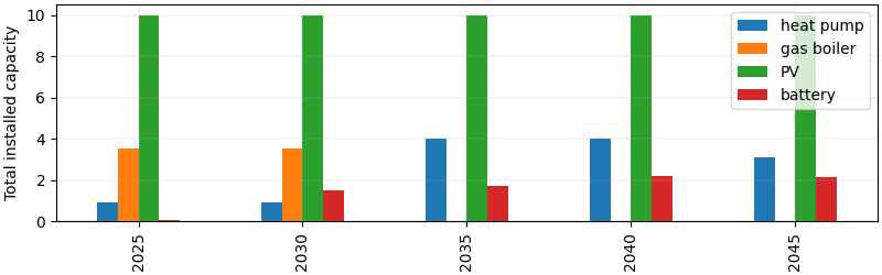
years = [2025, 2030, 2035, 2040, 2045]
invest.index = years
total.index = years

fig, ax1 = plt.subplots(
    1, 1, figsize=(8, 2.5), sharex=True, constrained_layout=True
)

total.plot(kind="bar", ax=ax1)
ax1.set_ylabel("Total installed capacity")
ax1.grid(True, linewidth=0.3, alpha=0.6)
ax1.legend(["heat pump", "gas boiler", "PV", "battery"], loc="best")

plt.show()


# Note: if you want to extract values for the flow, you have to change
# to_df() in the class Results() in this way:
#
#     # overwrite known indexes
#     index_type = tuple(dataset.index_set().subsets())[-1].name
#     match index_type:
#         case "TIMEPOINTS":
#             df.index = self.timeindex
#         case "TIMESTEPS":
#             # df.index = self.timeindex[:-1]
#             df.index = self.timeindex
#         case _:
#             df.index = df.index.get_level_values(-1)
#
# otherwise including the storage leads to Length mismatch Value Error
# why: no clue, something with TIMESTEPS and TIMEPOINTS for storage
#
# if you changed this you can use
# flows = results["flow"]
# to look at the time series