oemof.solph package
Submodules
oemof.solph.EnergySystem
solph version of oemof.network.energy_system
-
class
oemof.solph.network.energy_system.EnergySystem(**kwargs)[source]¶ Bases:
oemof.network.energy_system.EnergySystemA variant of the class EnergySystem from <oemof.network.network.energy_system.EnergySystem> specially tailored to solph.
In order to work in tandem with solph, instances of this class always use solph.GROUPINGS <oemof.solph.GROUPINGS>. If custom groupings are supplied via the groupings keyword argument, solph.GROUPINGS <oemof.solph.GROUPINGS> is prepended to those.
If you know what you are doing and want to use solph without solph.GROUPINGS <oemof.solph.GROUPINGS>, you can just use EnergySystem <oemof.network.network.energy_system.EnergySystem>` of oemof.network directly.
oemof.solph.Bus
solph version of oemof.network.bus
-
class
oemof.solph.network.bus.Bus(*args, **kwargs)[source]¶ Bases:
oemof.network.network.BusA balance object. Every node has to be connected to Bus.
Notes
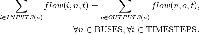
- The following sets, variables, constraints and objective parts are created
Creating sets, variables, constraints and parts of the objective function for Bus objects.
oemof.solph.Flow
solph version of oemof.network.Edge
-
class
oemof.solph.network.flow.Flow(**kwargs)[source]¶ Bases:
oemof.network.network.EdgeDefines a flow between two nodes.
Keyword arguments are used to set the attributes of this flow. Parameters which are handled specially are noted below. For the case where a parameter can be either a scalar or an iterable, a scalar value will be converted to a sequence containing the scalar value at every index. This sequence is then stored under the paramter’s key.
Parameters: nominal_value (numeric,
 ) – The nominal value of the flow. If this value is set the corresponding
optimization variable of the flow object will be bounded by this value
multiplied with min(lower bound)/max(upper bound).
) – The nominal value of the flow. If this value is set the corresponding
optimization variable of the flow object will be bounded by this value
multiplied with min(lower bound)/max(upper bound).max (numeric (iterable or scalar),
 ) – Normed maximum value of the flow. The flow absolute maximum will be
calculated by multiplying
) – Normed maximum value of the flow. The flow absolute maximum will be
calculated by multiplying nominal_valuewithmaxmin (numeric (iterable or scalar),
 ) – Normed minimum value of the flow (see
 max).fix (numeric (iterable or scalar),
 ) – Normed fixed value for the flow variable. Will be multiplied with the
nominal_valueto get the absolute value. Iffixedis set toTruethe flow variable will be fixed to fix * nominal_value, i.e. this value is set exogenous.positive_gradient (
dict, default: {‘ub’: None, ‘costs’: 0}) –A dictionary containing the following two keys:
- ‘ub’: numeric (iterable, scalar or None), the normed upper bound on the positive difference (flow[t-1] < flow[t]) of two consecutive flow values.
- ‘costs`: REMOVED!
negative_gradient (
dict, default: {‘ub’: None, ‘costs’: 0}) –A dictionary containing the following two keys:
- ‘ub’: numeric (iterable, scalar or None), the normed upper bound on the negative difference (flow[t-1] > flow[t]) of two consecutive flow values.
- ‘costs`: REMOVED!
summed_max (numeric,
 ) – Specific maximum value summed over all timesteps. Will be multiplied
with the nominal_value to get the absolute limit.
) – Specific maximum value summed over all timesteps. Will be multiplied
with the nominal_value to get the absolute limit.summed_min (numeric,
 ) – see above
variable_costs (numeric (iterable or scalar)) – The costs associated with one unit of the flow. If this is set the costs will be added to the objective expression of the optimization problem.
fixed (boolean) – Boolean value indicating if a flow is fixed during the optimization problem to its ex-ante set value. Used in combination with the
fix.investment (
Investment) – Object indicating if a nominal_value of the flow is determined by the optimization problem. Note: This will refer all attributes to an investment variable instead of to the nominal_value. The nominal_value should not be set (or set to None) if an investment object is used.nonconvex (
NonConvex) – If a nonconvex flow object is added here, the flow constraints will be altered significantly as the mathematical model for the flow will be different, i.e. constraint etc. fromNonConvexFlowwill be used instead ofFlow. Note: at the moment this does not work if the investment attribute is set .
Notes
- The following sets, variables, constraints and objective parts are created
FlowInvestmentFlow- (additionally if Investment object is present)
NonConvexFlow- (If nonconvex object is present, CAUTION: replaces
Flowclass and a MILP will be build)
Examples
Creating a fixed flow object:
>>> f = Flow(fix=[10, 4, 4], variable_costs=5)
>>> f.variable_costs[2]
5
>>> f.fix[2]
4
Creating a flow object with time-depended lower and upper bounds:
>>> f1 = Flow(min=[0.2, 0.3], max=0.99, nominal_value=100)
>>> f1.max[1]
0.99
Creating sets, variables, constraints and parts of the objective function for Flow objects.
-
class
oemof.solph.blocks.flow.Flow(*args, **kwargs)[source]¶ Bases:
pyomo.core.base.block.SimpleBlockFlow block with definitions for standard flows.
The following variables are created:
- negative_gradient :
- Difference of a flow in consecutive timesteps if flow is reduced indexed by NEGATIVE_GRADIENT_FLOWS, TIMESTEPS.
- positive_gradient :
- Difference of a flow in consecutive timesteps if flow is increased indexed by NEGATIVE_GRADIENT_FLOWS, TIMESTEPS.
The following sets are created: (-> see basic sets at
Model)- SUMMED_MAX_FLOWS
- A set of flows with the attribute
summed_maxbeing not None. - SUMMED_MIN_FLOWS
- A set of flows with the attribute
summed_minbeing not None. - NEGATIVE_GRADIENT_FLOWS
- A set of flows with the attribute
negative_gradientbeing not None. - POSITIVE_GRADIENT_FLOWS
- A set of flows with the attribute
positive_gradientbeing not None - INTEGER_FLOWS
- A set of flows where the attribute
integeris True (forces flow to only take integer values)
The following constraints are build:
- Flow max sum
om.Flow.summed_max[i, o] 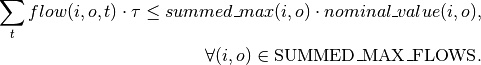
- Flow min sum
om.Flow.summed_min[i, o] 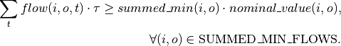
- Negative gradient constraint
om.Flow.negative_gradient_constr[i, o]:
- Positive gradient constraint
om.Flow.positive_gradient_constr[i, o]: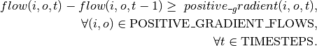
The following parts of the objective function are created:
- If
variable_costsare set by the user: 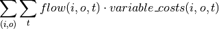
The expression can be accessed by
om.Flow.variable_costsand their value after optimization byom.Flow.variable_costs().
Creating sets, variables, constraints and parts of the objective function for Flow objects with investment option.
-
class
oemof.solph.blocks.investment_flow.InvestmentFlow(*args, **kwargs)[source]¶ Bases:
pyomo.core.base.block.SimpleBlockBlock for all flows with
Investmentbeing not None.See
oemof.solph.options.Investmentfor all parameters of the Investment class.See
oemof.solph.network.Flowfor all parameters of the Flow class.Variables
All InvestmentFlow are indexed by a starting and ending node
 , which is omitted in the following for the sake
of convenience. The following variables are created:
, which is omitted in the following for the sake
of convenience. The following variables are created:
Actual flow value (created in
oemof.solph.models.BaseModel).
Value of the investment variable, i.e. equivalent to the nominal value of the flows after optimization.

Binary variable for the status of the investment, if
nonconvexis True.
Constraints
Depending on the attributes of the InvestmentFlow and Flow, different constraints are created. The following constraint is created for all InvestmentFlow:
Upper bound for the flow value
Depeding on the attribute
nonconvex, the constraints for the bounds of the decision variable are different:nonconvex = False

nonconvex = True
For all InvestmentFlow (independent of the attribute
nonconvex), the following additional constraints are created, if the appropriate attribute of the Flow (seeoemof.solph.network.Flow) is set:fixis not NoneActual value constraint for investments with fixed flow values

min != 0Lower bound for the flow values

summed_max is not NoneUpper bound for the sum of all flow values (e.g. maximum full load hours)
summed_min is not NoneLower bound for the sum of all flow values (e.g. minimum full load hours)
Objective function
The part of the objective function added by the InvestmentFlow also depends on whether a convex or nonconvex InvestmentFlow is selected. The following parts of the objective function are created:
nonconvex = False
nonconvex = True
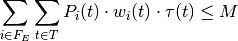
The total value of all costs of all InvestmentFlow can be retrieved calling
om.InvestmentFlow.investment_costs.expr().List of Variables (in csv table syntax)¶ symbol attribute explanation flow[n, o, t]Actual flow value invest[i, o]Invested flow capacity invest_status[i, o]Binary status of investment List of Variables (in rst table syntax):
symbol attribute explanation flow[n, o, t]Actual flow value invest[i, o]Invested flow capacity invest_status[i, o]Binary status of investment Grid table style:
symbol attribute explanation flow[n, o, t]Actual flow value invest[i, o]Invested flow capacity invest_status[i, o]Binary status of investment List of Parameters¶ symbol attribute explanation 
flows[i, o].investment.existingExisting flow capacity 
flows[i, o].investment.minimumMinimum investment capacity 
flows[i, o].investment.maximumMaximum investment capacity 
flows[i, o].investment.ep_costsVariable investment costs 
flows[i, o].investment.offsetFix investment costs flows[i, o].fix[t]Normed fixed value for the flow variable flows[i, o].max[t]Normed maximum value of the flow flows[i, o].min[t]Normed minimum value of the flow flows[i, o].summed_maxSpecific maximum of summed flow values (per installed capacity) flows[i, o].summed_minSpecific minimum of summed flow values (per installed capacity) 
timeincrement[t]Time step width for each time step Note
In case of a nonconvex investment flow (
nonconvex=True), the existing flow capacity needs to be zero.
At least, it is not tested yet, whether this works out, or makes any sense
at all.Note
See also
oemof.solph.network.Flow,oemof.solph.blocks.Flowandoemof.solph.options.Investment
Creating sets, variables, constraints and parts of the objective function for nonconvex Flow objects.
-
class
oemof.solph.blocks.non_convex_flow.NonConvexFlow(*args, **kwargs)[source]¶ Bases:
pyomo.core.base.block.SimpleBlockThe following sets are created: (-> see basic sets at
Model)- A set of flows with the attribute nonconvex of type
options.NonConvex.- MIN_FLOWS
- A subset of set NONCONVEX_FLOWS with the attribute min being not None in the first timestep.
- ACTIVITYCOSTFLOWS
- A subset of set NONCONVEX_FLOWS with the attribute activity_costs being not None.
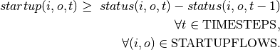
- STARTUPFLOWS
- A subset of set NONCONVEX_FLOWS with the attribute maximum_startups or startup_costs being not None.
- MAXSTARTUPFLOWS
- A subset of set STARTUPFLOWS with the attribute maximum_startups being not None.
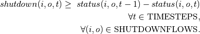
- SHUTDOWNFLOWS
- A subset of set NONCONVEX_FLOWS with the attribute maximum_shutdowns or shutdown_costs being not None.
- MAXSHUTDOWNFLOWS
- A subset of set SHUTDOWNFLOWS with the attribute maximum_shutdowns being not None.
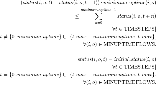
- MINUPTIMEFLOWS
- A subset of set NONCONVEX_FLOWS with the attribute minimum_uptime being not None.
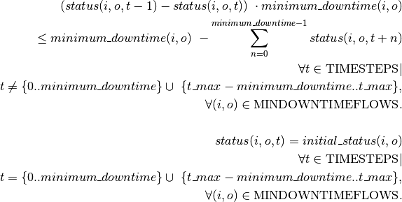
- MINDOWNTIMEFLOWS
- A subset of set NONCONVEX_FLOWS with the attribute minimum_downtime being not None.
- POSITIVE_GRADIENT_FLOWS
- A subset of set NONCONVEX_FLOWS with the attribute positive_gradient being not None.
- NEGATIVE_GRADIENT_FLOWS
- A subset of set NONCONVEX_FLOWS with the attribute negative_gradient being not None.
The following variables are created:
- Status variable (binary) om.NonConvexFlow.status:
- Variable indicating if flow is >= 0 indexed by FLOWS
- Startup variable (binary) om.NonConvexFlow.startup:
- Variable indicating startup of flow (component) indexed by STARTUPFLOWS
- Shutdown variable (binary) om.NonConvexFlow.shutdown:
- Variable indicating shutdown of flow (component) indexed by SHUTDOWNFLOWS
- Positive gradient (continuous) om.NonConvexFlow.positive_gradient:
- Variable indicating the positive gradient, i.e. the load increase between two consecutive timesteps, indexed by POSITIVE_GRADIENT_FLOWS
- Negative gradient (continuous) om.NonConvexFlow.negative_gradient:
- Variable indicating the negative gradient, i.e. the load decrease between two consecutive timesteps, indexed by NEGATIVE_GRADIENT_FLOWS
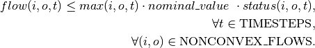
The following constraints are created:
- Minimum flow constraint om.NonConvexFlow.min[i,o,t]
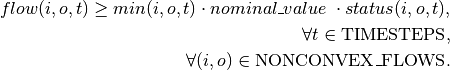
- Maximum flow constraint om.NonConvexFlow.max[i,o,t]
- Startup constraint om.NonConvexFlow.startup_constr[i,o,t]
- Maximum startups constraint
- om.NonConvexFlow.max_startup_constr[i,o,t]

- Shutdown constraint om.NonConvexFlow.shutdown_constr[i,o,t]
- Maximum shutdowns constraint
- om.NonConvexFlow.max_startup_constr[i,o,t]

- Minimum uptime constraint om.NonConvexFlow.uptime_constr[i,o,t]
- Minimum downtime constraint om.NonConvexFlow.downtime_constr[i,o,t]
- Positive gradient constraint
- om.NonConvexFlow.positive_gradient_constr[i, o]:

- flow(i, o, t-1) cdot status(i, o, t-1) geq positive_gradient(i, o, t), \ forall (i, o) in textrm{POSITIVE_GRADIENT_FLOWS}, \ forall t in textrm{TIMESTEPS}.
- Negative gradient constraint
- om.NonConvexFlow.negative_gradient_constr[i, o]:

The following parts of the objective function are created:
- If nonconvex.startup_costs is set by the user:

- If nonconvex.shutdown_costs is set by the user:

- If nonconvex.activity_costs is set by the user:

- If nonconvex.positive_gradient[“costs”] is set by the user:

- If nonconvex.negative_gradient[“costs”] is set by the user:

oemof.solph.Sink
solph version of oemof.network.Sink
oemof.solph.Source
solph version of oemof.network.Source
oemof.solph.Transformer
solph version of oemof.network.Transformer
-
class
oemof.solph.network.transformer.Transformer(*args, **kwargs)[source]¶ Bases:
oemof.network.network.TransformerA linear Transformer object with n inputs and n outputs.
Parameters: conversion_factors (dict) – Dictionary containing conversion factors for conversion of each flow. Keys are the connected bus objects. The dictionary values can either be a scalar or an iterable with length of time horizon for simulation. Examples
Defining an linear transformer:
>>> from oemof import solph
>>> bgas = solph.Bus(label='natural_gas')
>>> bcoal = solph.Bus(label='hard_coal')
>>> bel = solph.Bus(label='electricity')
>>> bheat = solph.Bus(label='heat')
>>> trsf = solph.Transformer(
...    label='pp_gas_1',
...    inputs={bgas: solph.Flow(), bcoal: solph.Flow()},
...    outputs={bel: solph.Flow(), bheat: solph.Flow()},
...    conversion_factors={bel: 0.3, bheat: 0.5,
...                        bgas: 0.8, bcoal: 0.2})
>>> print(sorted([x[1][5] for x in trsf.conversion_factors.items()]))
[0.2, 0.3, 0.5, 0.8]
>>> type(trsf)
<class 'oemof.solph.network.transformer.Transformer'>
>>> sorted([str(i) for i in trsf.inputs])
['hard_coal', 'natural_gas']
>>> trsf_new = solph.Transformer(
...    label='pp_gas_2',
...    inputs={bgas: solph.Flow()},
...    outputs={bel: solph.Flow(), bheat: solph.Flow()},
...    conversion_factors={bel: 0.3, bheat: 0.5})
>>> trsf_new.conversion_factors[bgas][3]
1
Notes
- The following sets, variables, constraints and objective parts are created
Creating sets, variables, constraints and parts of the objective function for Transformer objects.
-
class
oemof.solph.blocks.transformer.Transformer(*args, **kwargs)[source]¶ Bases:
pyomo.core.base.block.SimpleBlockBlock for the linear relation of nodes with type
TransformerThe following sets are created: (-> see basic sets at
Model)- TRANSFORMERS
- A set with all
Transformerobjects.
The following constraints are created:
- Linear relation
om.Transformer.relation[i,o,t] 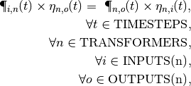
symbol attribute explanation 
flow[i, n, t] - Transformer
- inflow

flow[n, o, t] - Transformer
- outflow

conversion_factor[i, n, t] - Conversion
- efficiency
oemof.solph.components.ExtractionTurbineCHP
ExtractionTurbineCHP and associated individual constraints (blocks) and groupings.
-
class
oemof.solph.components.extraction_turbine_chp.ExtractionTurbineCHP(conversion_factor_full_condensation, *args, **kwargs)[source]¶ Bases:
oemof.solph.network.transformer.TransformerA CHP with an extraction turbine in a linear model. For more options see the
GenericCHPclass.One main output flow has to be defined and is tapped by the remaining flow. The conversion factors have to be defined for the maximum tapped flow ( full CHP mode) and for no tapped flow (full condensing mode). Even though it is possible to limit the variability of the tapped flow, so that the full condensing mode will never be reached.
Parameters: - conversion_factors (dict) – Dictionary containing conversion factors for conversion of inflow to specified outflow. Keys are output bus objects. The dictionary values can either be a scalar or a sequence with length of time horizon for simulation.
- conversion_factor_full_condensation (dict) – The efficiency of the main flow if there is no tapped flow. Only one key is allowed. Use one of the keys of the conversion factors. The key indicates the main flow. The other output flow is the tapped flow.
Notes
- The following sets, variables, constraints and objective parts are created
Examples
>>> from oemof import solph
>>> bel = solph.Bus(label='electricityBus')
>>> bth = solph.Bus(label='heatBus')
>>> bgas = solph.Bus(label='commodityBus')
>>> et_chp = solph.components.ExtractionTurbineCHP(
...    label='variable_chp_gas',
...    inputs={bgas: solph.Flow(nominal_value=10e10)},
...    outputs={bel: solph.Flow(), bth: solph.Flow()},
...    conversion_factors={bel: 0.3, bth: 0.5},
...    conversion_factor_full_condensation={bel: 0.5})
-
class
oemof.solph.components.extraction_turbine_chp.ExtractionTurbineCHPBlock(*args, **kwargs)[source]¶ Bases:
pyomo.core.base.block.SimpleBlockBlock for the linear relation of nodes with type
ExtractionTurbineCHPThe following two constraints are created:
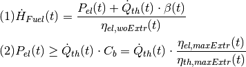
where
 is defined as:
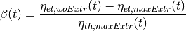
where the first equation is the result of the relation between the input flow and the two output flows, the second equation stems from how the two output flows relate to each other, and the symbols used are defined as follows (with Variables (V) and Parameters (P)):
symbol attribute type explanation 
flow[i, n, t] V fuel input flow 
flow[n, main_output, t] V electric power 
flow[n, tapped_output, t] V thermal output main_flow_loss_index[n, t] P power loss index 
conversion_factor_full_condensation[n, t] P - electric efficiency
- without heat extraction

conversion_factors[main_output][n, t] P - electric efficiency
- with max heat extraction

conversion_factors[tapped_output][n, t] P - thermal efficiency with
- maximal heat extraction
-
CONSTRAINT_GROUP= True
oemof.solph.components.GenericCHP
GenericCHP and associated individual constraints (blocks) and groupings.
-
class
oemof.solph.components.generic_chp.GenericCHP(*args, **kwargs)[source]¶ Bases:
oemof.network.network.TransformerComponent GenericCHP to model combined heat and power plants.
Can be used to model (combined cycle) extraction or back-pressure turbines and used a mixed-integer linear formulation. Thus, it induces more computational effort than the ExtractionTurbineCHP for the benefit of higher accuracy.
The full set of equations is described in: Mollenhauer, E., Christidis, A. & Tsatsaronis, G. Evaluation of an energy- and exergy-based generic modeling approach of combined heat and power plants Int J Energy Environ Eng (2016) 7: 167. https://doi.org/10.1007/s40095-016-0204-6
For a general understanding of (MI)LP CHP representation, see: Fabricio I. Salgado, P. Short - Term Operation Planning on Cogeneration Systems: A Survey Electric Power Systems Research (2007) Electric Power Systems Research Volume 78, Issue 5, May 2008, Pages 835-848 https://doi.org/10.1016/j.epsr.2007.06.001
Note
An adaption for the flow parameter H_L_FG_share_max has been made to set the flue gas losses at maximum heat extraction H_L_FG_max as share of the fuel flow H_F e.g. for combined cycle extraction turbines. The flow parameter H_L_FG_share_min can be used to set the flue gas losses at minimum heat extraction H_L_FG_min as share of the fuel flow H_F e.g. for motoric CHPs. The boolean component parameter back_pressure can be set to model back-pressure characteristics.
Also have a look at the examples on how to use it.
Parameters: - fuel_input (dict) – Dictionary with key-value-pair of oemof.Bus and oemof.Flow object for the fuel input.
- electrical_output (dict) – Dictionary with key-value-pair of oemof.Bus and oemof.Flow object for the electrical output. Related parameters like P_max_woDH are passed as attributes of the oemof.Flow object.
- heat_output (dict) – Dictionary with key-value-pair of oemof.Bus and oemof.Flow object for the heat output. Related parameters like Q_CW_min are passed as attributes of the oemof.Flow object.
- Beta (list of numerical values) – Beta values in same dimension as all other parameters (length of optimization period).
- back_pressure (boolean) – Flag to use back-pressure characteristics. Set to True and Q_CW_min to zero for back-pressure turbines. See paper above for more information.
Note
- The following sets, variables, constraints and objective parts are created
Examples
>>> from oemof import solph
>>> bel = solph.Bus(label='electricityBus')
>>> bth = solph.Bus(label='heatBus')
>>> bgas = solph.Bus(label='commodityBus')
>>> ccet = solph.components.GenericCHP(
...    label='combined_cycle_extraction_turbine',
...    fuel_input={bgas: solph.Flow(
...        H_L_FG_share_max=[0.183])},
...    electrical_output={bel: solph.Flow(
...        P_max_woDH=[155.946],
...        P_min_woDH=[68.787],
...        Eta_el_max_woDH=[0.525],
...        Eta_el_min_woDH=[0.444])},
...    heat_output={bth: solph.Flow(
...        Q_CW_min=[10.552])},
...    Beta=[0.122], back_pressure=False)
>>> type(ccet)
<class 'oemof.solph.components.generic_chp.GenericCHP'>
-
alphas¶ Compute or return the _alphas attribute.
-
class
oemof.solph.components.generic_chp.GenericCHPBlock(*args, **kwargs)[source]¶ Bases:
pyomo.core.base.block.SimpleBlockBlock for the relation of the
 nodes with
type class:.GenericCHP.
nodes with
type class:.GenericCHP.The following constraints are created:
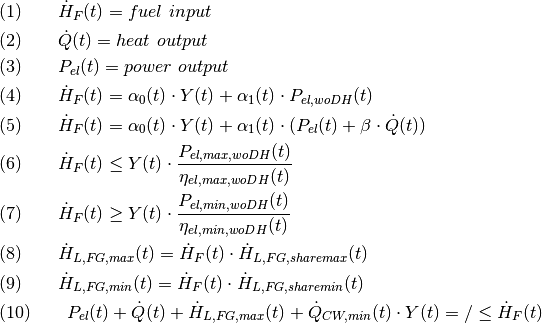
where
 depends on the CHP being back pressure or not.
The coefficients
 and
and  can be determined given the efficiencies maximal/minimal load:
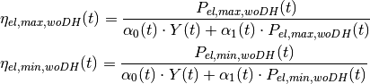
For the attribute
 being not None,
e.g. for a motoric CHP, the following is created:Constraint:
being not None,
e.g. for a motoric CHP, the following is created:Constraint:![&
(11)\qquad P_{el}(t) + \dot{Q}(t) + \dot{H}_{L,FG,min}(t) +
\dot{Q}_{CW, min}(t) \cdot Y(t) \geq \dot{H}_F(t)\\[10pt]](../_images/math/042acad6b4fc164679a9a283618487cc30ac9bd3.png)
The symbols used are defined as follows (with Variables (V) and Parameters (P)):
math. symbol attribute type explanation 
H_F[n,t] V - input of enthalpy
- through fuel input
P[n,t] V - provided
- electric power

P_woDH[n,t] V - electric power without
- district heating

P_min_woDH[n,t] P - min. electric power
- without district heating

P_max_woDH[n,t] P - max. electric power
- without district heating

Q[n,t] V provided heat 
Q_CW_min[n,t] P - minimal therm. condenser
- load to cooling water
H_L_FG_min[n,t] V - flue gas enthalpy loss
- at min heat extraction

H_L_FG_max[n,t] V - flue gas enthalpy loss
- at max heat extraction
H_L_FG_share_min[n,t] P - share of flue gas loss
- at min heat extraction
H_L_FG_share_max[n,t] P - share of flue gas loss
- at max heat extraction

Y[n,t] V - status variable
- on/off
n.alphas[0][n,t] P - coefficient
- describing efficiency
n.alphas[1][n,t] P - coefficient
- describing efficiency
Beta[n,t] P power loss index 
Eta_el_min_woDH[n,t] P - el. eff. at min. fuel
- flow w/o distr. heating

Eta_el_max_woDH[n,t] P - el. eff. at max. fuel
- flow w/o distr. heating
-
CONSTRAINT_GROUP= True
oemof.solph.components.GenericStorage
GenericStorage and associated individual constraints (blocks) and groupings.
-
class
oemof.solph.components.generic_storage.GenericInvestmentStorageBlock(*args, **kwargs)[source]¶ Bases:
pyomo.core.base.block.SimpleBlockBlock for all storages with
Investmentbeing not None. Seeoemof.solph.options.Investmentfor all parameters of the Investment class.Variables
All Storages are indexed by
, which is omitted in the following
for the sake of convenience.
The following variables are created as attributes of
om.InvestmentStorage:
Inflow of the storage (created in
oemof.solph.models.BaseModel).
Outflow of the storage (created in
oemof.solph.models.BaseModel).
Current storage content (Absolute level of stored energy).

Invested (nominal) capacity of the storage.

Initial storage content (before timestep 0).
Binary variable for the status of the investment, if
nonconvexis True.
Constraints
The following constraints are created for all investment storages:
Storage balance (Same as forGenericStorageBlock)
Depending on the attribute
nonconvex, the constraints for the bounds of the decision variable are different:nonconvex = False

nonconvex = True

The following constraints are created depending on the attributes of the
components.GenericStorage:initial_storage_level is NoneConstraint for a variable initial storage content:

initial_storage_level is not NoneAn initial value for the storage content is given:

balanced=TrueThe energy content of storage of the first and the last timestep are set equal:
invest_relation_input_capacity is not NoneConnect the invest variables of the storage and the input flow:

invest_relation_output_capacity is not NoneConnect the invest variables of the storage and the output flow:

invest_relation_input_output is not NoneConnect the invest variables of the input and the output flow:

max_storage_levelRule for upper bound constraint for the storage content:
min_storage_levelRule for lower bound constraint for the storage content:
Objective function
The part of the objective function added by the investment storages also depends on whether a convex or nonconvex investment option is selected. The following parts of the objective function are created:
nonconvex = False
nonconvex = True
The total value of all investment costs of all InvestmentStorages can be retrieved calling
om.GenericInvestmentStorageBlock.investment_costs.expr().List of Variables¶ symbol attribute explanation flow[i[n], n, t]Inflow of the storage flow[n, o[n], t]Outlfow of the storage storage_content[n, t]Current storage content (current absolute stored energy) invest[n, t]Invested (nominal) capacity of the storage init_cap[n]Initial storage capacity (before timestep 0) invest_status[i, o]Binary variable for the status of investment 
InvestmentFlow.invest[i[n], n]Invested (nominal) inflow (Investmentflow) 
InvestmentFlow.invest[n, o[n]]Invested (nominal) outflow (Investmentflow) List of Parameters¶ symbol attribute explanation 
flows[i, o].investment.existing Existing storage capacity 
flows[i, o].investment.minimum Minimum investment value 
flows[i, o].investment.maximum Maximum investment value 
flows[i[n], n].investment.existing Existing inflow capacity 
flows[n, o[n]].investment.existing Existing outlfow capacity flows[i, o].investment.ep_costs Variable investment costs flows[i, o].investment.offset Fix investment costs 
invest_relation_input_capacityRelation of storage capacity and nominal inflow 
invest_relation_output_capacityRelation of storage capacity and nominal outflow 
invest_relation_input_outputRelation of nominal in- and outflow 
loss_rate[t] Fraction of lost energy as share of per time unit
fixed_losses_relative[t] Fixed loss of energy relative to  per time unit
fixed_losses_absolute[t] Absolute fixed loss of energy per time unit 
inflow_conversion_factor[t] Conversion factor (i.e. efficiency) when storing energy 
outflow_conversion_factor[t] Conversion factor when (i.e. efficiency) taking stored energy 
initial_storage_level Initial relativ storage content (before timestep 0) 
flows[i, o].max[t] Normed maximum value of storage content 
flows[i, o].min[t] Normed minimum value of storage content Duration of time step 
Time unit of losses ,
, and timeincrement -
CONSTRAINT_GROUP= True
-
class
oemof.solph.components.generic_storage.GenericStorage(*args, max_storage_level=1, min_storage_level=0, **kwargs)[source]¶ Bases:
oemof.network.network.NodeComponent GenericStorage to model with basic characteristics of storages.
The GenericStorage is designed for one input and one output.
Parameters: - nominal_storage_capacity (numeric,
 ) – Absolute nominal capacity of the storage
 - invest_relation_input_capacity (numeric or None, ) – Ratio between the investment variable of the input Flow and the
investment variable of the storage:
- invest_relation_output_capacity (numeric or None, ) – Ratio between the investment variable of the output Flow and the
investment variable of the storage:
- invest_relation_input_output (numeric or None, ) – Ratio between the investment variable of the output Flow and the
investment variable of the input flow. This ratio used to fix the
flow investments to each other.
Values < 1 set the input flow lower than the output and > 1 will
set the input flow higher than the output flow. If None no relation
will be set:
- initial_storage_level (numeric, ) – The relative storage content in the timestep before the first
time step of optimization (between 0 and 1).
- balanced (boolean) – Couple storage level of first and last time step. (Total inflow and total outflow are balanced.)
- loss_rate (numeric (iterable or scalar)) – The relative loss of the storage content per time unit.
- fixed_losses_relative (numeric (iterable or scalar), ) – Losses independent of state of charge between two consecutive
timesteps relative to nominal storage capacity.
- fixed_losses_absolute (numeric (iterable or scalar), ) – Losses independent of state of charge and independent of
nominal storage capacity between two consecutive timesteps.
- inflow_conversion_factor (numeric (iterable or scalar), ) – The relative conversion factor, i.e. efficiency associated with the
inflow of the storage.
- outflow_conversion_factor (numeric (iterable or scalar), ) – see: inflow_conversion_factor
- min_storage_level (numeric (iterable or scalar),
 ) – The normed minimum storage content as fraction of the
nominal storage capacity (between 0 and 1).
To set different values in every time step use a sequence.
) – The normed minimum storage content as fraction of the
nominal storage capacity (between 0 and 1).
To set different values in every time step use a sequence. - max_storage_level (numeric (iterable or scalar),
 ) – see: min_storage_level
 - investment (
oemof.solph.options.Investmentobject) – Object indicating if a nominal_value of the flow is determined by the optimization problem. Note: This will refer all attributes to an investment variable instead of to the nominal_storage_capacity. The nominal_storage_capacity should not be set (or set to None) if an investment object is used.
Notes
- The following sets, variables, constraints and objective parts are created
GenericStorageBlock(if no Investment object present)GenericInvestmentStorageBlock(if Investment object present)
Examples
Basic usage examples of the GenericStorage with a random selection of attributes. See the Flow class for all Flow attributes.
>>> from oemof import solph
>>> my_bus = solph.Bus('my_bus')
>>> my_storage = solph.components.GenericStorage(
...     label='storage',
...     nominal_storage_capacity=1000,
...     inputs={my_bus: solph.Flow(nominal_value=200, variable_costs=10)},
...     outputs={my_bus: solph.Flow(nominal_value=200)},
...     loss_rate=0.01,
...     initial_storage_level=0,
...     max_storage_level = 0.9,
...     inflow_conversion_factor=0.9,
...     outflow_conversion_factor=0.93)
>>> my_investment_storage = solph.components.GenericStorage(
...     label='storage',
...     investment=solph.Investment(ep_costs=50),
...     inputs={my_bus: solph.Flow()},
...     outputs={my_bus: solph.Flow()},
...     loss_rate=0.02,
...     initial_storage_level=None,
...     invest_relation_input_capacity=1/6,
...     invest_relation_output_capacity=1/6,
...     inflow_conversion_factor=1,
...     outflow_conversion_factor=0.8)
- nominal_storage_capacity (numeric,
-
class
oemof.solph.components.generic_storage.GenericStorageBlock(*args, **kwargs)[source]¶ Bases:
pyomo.core.base.block.SimpleBlockStorage without an
Investmentobject.The following sets are created: (-> see basic sets at
Model)- STORAGES
- A set with all
Storageobjects, which do not have an - attr:investment of type
Investment.
- A set with all
- STORAGES_BALANCED
- A set of all
GenericStorageobjects, with ‘balanced’ attribute set to True. - STORAGES_WITH_INVEST_FLOW_REL
- A set with all
Storageobjects with two investment flows coupled with the ‘invest_relation_input_output’ attribute.
The following variables are created:
- storage_content
- Storage content for every storage and timestep. The value for the storage content at the beginning is set by the parameter initial_storage_level or not set if initial_storage_level is None. The variable of storage s and timestep t can be accessed by: om.Storage.storage_content[s, t]
The following constraints are created:
- Set storage_content of last time step to one at t=0 if balanced == True
- Storage balance
om.Storage.balance[n, t] 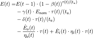
- Connect the invest variables of the input and the output flow.
symbol explanation attribute energy currently stored storage_content nominal capacity of the energy storage nominal_storage_capacity state before initial time step initial_storage_level minimum allowed storage min_storage_level[t] maximum allowed storage max_storage_level[t] fraction of lost energy as share of
per time unitloss_rate[t] fixed loss of energy relative to per
time unitfixed_losses_relative[t] absolute fixed loss of energy per time unit fixed_losses_absolute[t] 
energy flowing in inputs 
energy flowing out outputs conversion factor (i.e. efficiency) when storing energy inflow_conversion_factor[t] conversion factor when (i.e. efficiency) taking stored energy outflow_conversion_factor[t] duration of time step time unit of losses ,
and
timeincrement
The following parts of the objective function are created:
Nothing added to the objective function.
-
CONSTRAINT_GROUP= True
oemof.solph.components.OffsetTransformer
OffsetTransformer and associated individual constraints (blocks) and groupings.
-
class
oemof.solph.components.offset_transformer.OffsetTransformer(*args, **kwargs)[source]¶ Bases:
oemof.network.network.TransformerAn object with one input and one output.
Parameters: coefficients (tuple) – Tuple containing the first two polynomial coefficients i.e. the y-intersection and slope of a linear equation. The tuple values can either be a scalar or a sequence with length of time horizon for simulation. Notes
- The sets, variables, constraints and objective parts are created
Examples
>>> from oemof import solph
>>> bel = solph.Bus(label='bel')
>>> bth = solph.Bus(label='bth')
>>> ostf = solph.components.OffsetTransformer(
...    label='ostf',
...    inputs={bel: solph.Flow(
...        nominal_value=60, min=0.5, max=1.0,
...        nonconvex=solph.NonConvex())},
...    outputs={bth: solph.Flow()},
...    coefficients=(20, 0.5))
>>> type(ostf)
<class 'oemof.solph.components.offset_transformer.OffsetTransformer'>
-
class
oemof.solph.components.offset_transformer.OffsetTransformerBlock(*args, **kwargs)[source]¶ Bases:
pyomo.core.base.block.SimpleBlockBlock for the relation of nodes with type
OffsetTransformerThe following constraints are created:

Variables (V) and Parameters (P)¶ symbol attribute type explanation 
flow[n, o, t] V Power of output 
flow[i, n, t] V Power of input 
status[i, n, t] V binary status variable of nonconvex input flow 
coefficients[1][n, t] P linear coefficient 1 (slope) 
coefficients[0][n, t] P linear coefficient 0 (y-intersection) -
CONSTRAINT_GROUP= True
-
oemof.solph.constraints module
Additional constraints to be used in an oemof energy model.
-
oemof.solph.constraints.equate_variables(model, var1, var2, factor1=1, name=None)[source]¶ Adds a constraint to the given model that set two variables to equal adaptable by a factor.
The following constraints are build:

Parameters: - var1 (pyomo.environ.Var) – First variable, to be set to equal with Var2 and multiplied with factor1.
- var2 (pyomo.environ.Var) – Second variable, to be set equal to (Var1 * factor1).
- factor1 (float) – Factor to define the proportion between the variables.
- name (str) – Optional name for the equation e.g. in the LP file. By default the name is: equate + string representation of var1 and var2.
- model (oemof.solph.Model) – Model to which the constraint is added.
Examples
The following example shows how to define a transmission line in the investment mode by connecting both investment variables. Note that the equivalent periodical costs (epc) of the line are 40. You could also add them to one line and set them to 0 for the other line.
>>> import pandas as pd
>>> from oemof import solph
>>> date_time_index = pd.date_range('1/1/2012', periods=5, freq='H')
>>> energysystem = solph.EnergySystem(timeindex=date_time_index)
>>> bel1 = solph.Bus(label='electricity1')
>>> bel2 = solph.Bus(label='electricity2')
>>> energysystem.add(bel1, bel2)
>>> energysystem.add(solph.Transformer(
...    label='powerline_1_2',
...    inputs={bel1: solph.Flow()},
...    outputs={bel2: solph.Flow(
...        investment=solph.Investment(ep_costs=20))}))
>>> energysystem.add(solph.Transformer(
...    label='powerline_2_1',
...    inputs={bel2: solph.Flow()},
...   outputs={bel1: solph.Flow(
...       investment=solph.Investment(ep_costs=20))}))
>>> om = solph.Model(energysystem)
>>> line12 = energysystem.groups['powerline_1_2']
>>> line21 = energysystem.groups['powerline_2_1']
>>> solph.constraints.equate_variables(
...    om,
...    om.InvestmentFlow.invest[line12, bel2],
...    om.InvestmentFlow.invest[line21, bel1])
-
oemof.solph.constraints.limit_active_flow_count(model, constraint_name, flows, lower_limit=0, upper_limit=None)[source]¶ Set limits (lower and/or upper) for the number of concurrently active NonConvex flows. The flows are given as a list.
Total actual counts after optimization can be retrieved calling the
om.oemof.solph.Model.$(constraint_name)_count().Parameters: - model (oemof.solph.Model) – Model to which constraints are added
- constraint_name (string) – name for the constraint
- flows (list of flows) – flows (have to be NonConvex) in the format [(in, out)]
- lower_limit (integer) – minimum number of active flows in the list
- upper_limit (integer) – maximum number of active flows in the list
Returns: the updated model
Note
Flow objects required to be NonConvex
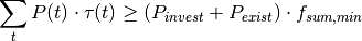
Constraint:
With F being the set of considered flows and T being the set of time steps.
The symbols used are defined as follows (with Variables (V) and Parameters (P)):
math. symbol type explanation 
V status (0 or 1) of the flow
at time step 

P lower_limit 
P lower_limit
-
oemof.solph.constraints.limit_active_flow_count_by_keyword(model, keyword, lower_limit=0, upper_limit=None)[source]¶ This wrapper for limit_active_flow_count allows to set limits to the count of concurrently active flows by using a keyword instead of a list. The constraint will be named $(keyword)_count.
Parameters: - model (oemof.solph.Model) – Model to which constraints are added
- keyword (string) – keyword to consider (searches all NonConvexFlows)
- lower_limit (integer) – minimum number of active flows having the keyword
- upper_limit (integer) – maximum number of active flows having the keyword
Returns: the updated model
See also
limit_active_flow_count(),constraint_name(),flows()
-
oemof.solph.constraints.emission_limit(om, flows=None, limit=None)[source]¶ Short handle for generic_integral_limit() with keyword=”emission_factor”.
Note
Flow objects required an attribute “emission_factor”!
-
oemof.solph.constraints.generic_integral_limit(om, keyword, flows=None, limit=None)[source]¶ Set a global limit for flows weighted by attribute called keyword. The attribute named by keyword has to be added to every flow you want to take into account.
Total value of keyword attributes after optimization can be retrieved calling the
om.oemof.solph.Model.integral_limit_${keyword}().Parameters: - om (oemof.solph.Model) – Model to which constraints are added.
- flows (dict) – Dictionary holding the flows that should be considered in constraint. Keys are (source, target) objects of the Flow. If no dictionary is given all flows containing the keyword attribute will be used.
- keyword (string) – attribute to consider
- limit (numeric) – Absolute limit of keyword attribute for the energy system.
Note
Flow objects required an attribute named like keyword!
Constraint:
With F_I being the set of flows considered for the integral limit and T being the set of time steps.
The symbols used are defined as follows (with Variables (V) and Parameters (P)):
math. symbol type explanation 
V power flow at time step 
P weight given to Flow named according to keyword P width of time step 
P global limit given by keyword limit Examples
>>> import pandas as pd
>>> from oemof import solph
>>> date_time_index = pd.date_range('1/1/2012', periods=5, freq='H')
>>> energysystem = solph.EnergySystem(timeindex=date_time_index)
>>> bel = solph.Bus(label='electricityBus')
>>> flow1 = solph.Flow(nominal_value=100, my_factor=0.8)
>>> flow2 = solph.Flow(nominal_value=50)
>>> src1 = solph.Source(label='source1', outputs={bel: flow1})
>>> src2 = solph.Source(label='source2', outputs={bel: flow2})
>>> energysystem.add(bel, src1, src2)
>>> model = solph.Model(energysystem)
>>> flow_with_keyword = {(src1, bel): flow1, }
>>> model = solph.constraints.generic_integral_limit(
...     model, "my_factor", flow_with_keyword, limit=777)
-
oemof.solph.constraints.additional_investment_flow_limit(model, keyword, limit=None)[source]¶ Global limit for investment flows weighted by an attribute keyword.
This constraint is only valid for Flows not for components such as an investment storage.
The attribute named by keyword has to be added to every Investment attribute of the flow you want to take into account. Total value of keyword attributes after optimization can be retrieved calling the
oemof.solph.Model.invest_limit_${keyword}().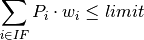
With IF being the set of InvestmentFlows considered for the integral limit.
The symbols used are defined as follows (with Variables (V) and Parameters (P)):
symbol attribute type explanation 
InvestmentFlow.invest[i, o] V installed capacity of investment flow 
keyword P weight given to investment flow named according to keyword 
limit P global limit given by keyword limit Parameters: - model (oemof.solph.Model) – Model to which constraints are added.
- keyword (attribute to consider) – All flows with Investment attribute containing the keyword will be used.
- limit (numeric) – Global limit of keyword attribute for the energy system.
Note
The Investment attribute of the considered (Investment-)flows requires an attribute named like keyword!
Examples
>>> import pandas as pd
>>> from oemof import solph
>>> date_time_index = pd.date_range('1/1/2020', periods=5, freq='H')
>>> es = solph.EnergySystem(timeindex=date_time_index)
>>> bus = solph.Bus(label='bus_1')
>>> sink = solph.Sink(label="sink", inputs={bus:
...     solph.Flow(nominal_value=10, fix=[10, 20, 30, 40, 50])})
>>> src1 = solph.Source(label='source_0', outputs={bus: solph.Flow(
...     investment=solph.Investment(ep_costs=50, space=4))})
>>> src2 = solph.Source(label='source_1', outputs={bus: solph.Flow(
...     investment=solph.Investment(ep_costs=100, space=1))})
>>> es.add(bus, sink, src1, src2)
>>> model = solph.Model(es)
>>> model = solph.constraints.additional_investment_flow_limit(
...     model, "space", limit=1500)
>>> a = model.solve(solver="cbc")
>>> int(round(model.invest_limit_space()))
1500
-
oemof.solph.constraints.investment_limit(model, limit=None)[source]¶ Set an absolute limit for the total investment costs of an investment optimization problem:
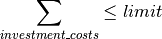
Parameters: - model (oemof.solph.Model) – Model to which the constraint is added
- limit (float) – Absolute limit of the investment (i.e. RHS of constraint)
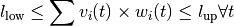
Adds a constraint to the given model that restricts the weighted sum of variables to a corridor.
The following constraints are build:
Parameters: - model (oemof.solph.Model) – Model to which the constraint is added.
- limit_name (string) – Name of the constraint to create
- quantity (pyomo.core.base.var.IndexedVar) – Shared Pyomo variable for all components of a type.
- components (list of components) – list of components of the same type
- weights (list of numeric values) – has to have the same length as the list of components
- lower_limit (numeric) – the lower limit
- upper_limit (numeric) – the lower limit
Examples
The constraint can e.g. be used to define a common storage that is shared between parties but that do not exchange energy on balance sheet. Thus, every party has their own bus and storage, respectively, to model the energy flow. However, as the physical storage is shared, it has a common limit.
>>> import pandas as pd
>>> from oemof import solph
>>> date_time_index = pd.date_range('1/1/2012', periods=5, freq='H')
>>> energysystem = solph.EnergySystem(timeindex=date_time_index)
>>> b1 = solph.Bus(label="Party1Bus")
>>> b2 = solph.Bus(label="Party2Bus")
>>> storage1 = solph.components.GenericStorage(
...     label="Party1Storage",
...     nominal_storage_capacity=5,
...     inputs={b1: solph.Flow()},
...     outputs={b1: solph.Flow()})
>>> storage2 = solph.components.GenericStorage(
...     label="Party2Storage",
...     nominal_storage_capacity=5,
...     inputs={b1: solph.Flow()},
...     outputs={b1: solph.Flow()})
>>> energysystem.add(b1, b2, storage1, storage2)
>>> components = [storage1, storage2]
>>> model = solph.Model(energysystem)
>>> solph.constraints.shared_limit(
...    model,
...    model.GenericStorageBlock.storage_content,
...    "limit_storage", components,
...    [1, 1], upper_limit=5)
oemof.solph.console_scripts module
This module can be used to check the installation.
This is not an illustrated example.
oemof.solph.custom.ElectricalLine
In-development electrical line components.
-
class
oemof.solph.custom.electrical_line.ElectricalBus(*args, **kwargs)[source]¶ Bases:
oemof.solph.network.bus.BusA electrical bus object. Every node has to be connected to Bus. This Bus is used in combination with ElectricalLine objects for linear optimal power flow (lopf) calculations.
Parameters: - slack (boolean) – If True Bus is slack bus for network
- v_max (numeric) – Maximum value of voltage angle at electrical bus
- v_min (numeric) – Mininum value of voltag angle at electrical bus
- Note (This component is experimental. Use it with care.)
Notes
- The following sets, variables, constraints and objective parts are created
- The objects are also used inside:
-
class
oemof.solph.custom.electrical_line.ElectricalLine(*args, **kwargs)[source]¶ Bases:
oemof.solph.network.flow.FlowAn ElectricalLine to be used in linear optimal power flow calculations. based on angle formulation. Check out the Notes below before using this component!
Parameters: - reactance (float or array of floats) – Reactance of the line to be modelled
- Note (This component is experimental. Use it with care.)
Notes
- To use this object the connected buses need to be of the type
ElectricalBus. - It does not work together with flows that have set the attr.`nonconvex`, i.e. unit commitment constraints are not possible
- Input and output of this component are set equal, therefore just use either only the input or the output to parameterize.
- Default attribute min of in/outflows is overwritten by -1 if not set differently by the user
- The following sets, variables, constraints and objective parts are created
-
class
oemof.solph.custom.electrical_line.ElectricalLineBlock(*args, **kwargs)[source]¶ Bases:
pyomo.core.base.block.SimpleBlockBlock for the linear relation of nodes with type class:.ElectricalLine
Note: This component is experimental. Use it with care.
The following constraints are created:
- Linear relation
om.ElectricalLine.electrical_flow[n,t] 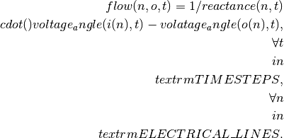
TODO: Add equate constraint of flows
The following variable are created:
TODO: Add voltage angle variable
TODO: Add fix slack bus voltage angle to zero constraint / bound
TODO: Add tests
-
CONSTRAINT_GROUP= True
- Linear relation
oemof.solph.custom.GenericCAES
In-development generic compressed air energy storage.
-
class
oemof.solph.custom.generic_caes.GenericCAES(*args, **kwargs)[source]¶ Bases:
oemof.network.network.TransformerComponent GenericCAES to model arbitrary compressed air energy storages.
The full set of equations is described in: Kaldemeyer, C.; Boysen, C.; Tuschy, I. A Generic Formulation of Compressed Air Energy Storage as Mixed Integer Linear Program – Unit Commitment of Specific Technical Concepts in Arbitrary Market Environments Materials Today: Proceedings 00 (2018) 0000–0000 [currently in review]
Parameters: - electrical_input (dict) – Dictionary with key-value-pair of oemof.Bus and oemof.Flow object for the electrical input.
- fuel_input (dict) – Dictionary with key-value-pair of oemof.Bus and oemof.Flow object for the fuel input.
- electrical_output (dict) – Dictionary with key-value-pair of oemof.Bus and oemof.Flow object for the electrical output.
- Note (This component is experimental. Use it with care.)
Notes
- The following sets, variables, constraints and objective parts are created
GenericCAES
TODO: Add description for constraints. See referenced paper until then!
Examples
>>> from oemof import solph
>>> bel = solph.Bus(label='bel')
>>> bth = solph.Bus(label='bth')
>>> bgas = solph.Bus(label='bgas')
>>> # dictionary with parameters for a specific CAES plant
>>> concept = {
...    'cav_e_in_b': 0,
...    'cav_e_in_m': 0.6457267578,
...    'cav_e_out_b': 0,
...    'cav_e_out_m': 0.3739636077,
...    'cav_eta_temp': 1.0,
...    'cav_level_max': 211.11,
...    'cmp_p_max_b': 86.0918959849,
...    'cmp_p_max_m': 0.0679999932,
...    'cmp_p_min': 1,
...    'cmp_q_out_b': -19.3996965679,
...    'cmp_q_out_m': 1.1066036114,
...    'cmp_q_tes_share': 0,
...    'exp_p_max_b': 46.1294016678,
...    'exp_p_max_m': 0.2528340303,
...    'exp_p_min': 1,
...    'exp_q_in_b': -2.2073411014,
...    'exp_q_in_m': 1.129249765,
...    'exp_q_tes_share': 0,
...    'tes_eta_temp': 1.0,
...    'tes_level_max': 0.0}
>>> # generic compressed air energy storage (caes) plant
>>> caes = solph.custom.GenericCAES(
...    label='caes',
...    electrical_input={bel: solph.Flow()},
...    fuel_input={bgas: solph.Flow()},
...    electrical_output={bel: solph.Flow()},
...    params=concept, fixed_costs=0)
>>> type(caes)
<class 'oemof.solph.custom.generic_caes.GenericCAES'>
-
class
oemof.solph.custom.generic_caes.GenericCAESBlock(*args, **kwargs)[source]¶ Bases:
pyomo.core.base.block.SimpleBlockBlock for nodes of class:.GenericCAES.
Note: This component is experimental. Use it with care.
The following constraints are created:
![&
(1) \qquad P_{cmp}(t) = electrical\_input (t)
\quad \forall t \in T \\
&
(2) \qquad P_{cmp\_max}(t) = m_{cmp\_max} \cdot CAS_{fil}(t-1)
+ b_{cmp\_max}
\quad \forall t \in\left[1, t_{max}\right] \\
&
(3) \qquad P_{cmp\_max}(t) = b_{cmp\_max}
\quad \forall t \notin\left[1, t_{max}\right] \\
&
(4) \qquad P_{cmp}(t) \leq P_{cmp\_max}(t)
\quad \forall t \in T \\
&
(5) \qquad P_{cmp}(t) \geq P_{cmp\_min} \cdot ST_{cmp}(t)
\quad \forall t \in T \\
&
(6) \qquad P_{cmp}(t) = m_{cmp\_max} \cdot CAS_{fil\_max}
+ b_{cmp\_max} \cdot ST_{cmp}(t)
\quad \forall t \in T \\
&
(7) \qquad \dot{Q}_{cmp}(t) =
m_{cmp\_q} \cdot P_{cmp}(t) + b_{cmp\_q} \cdot ST_{cmp}(t)
\quad \forall t \in T \\
&
(8) \qquad \dot{Q}_{cmp}(t) = \dot{Q}_{cmp_out}(t)
+ \dot{Q}_{tes\_in}(t)
\quad \forall t \in T \\
&
(9) \qquad r_{cmp\_tes} \cdot\dot{Q}_{cmp\_out}(t) =
\left(1-r_{cmp\_tes}\right) \dot{Q}_{tes\_in}(t)
\quad \forall t \in T \\
&
(10) \quad\; P_{exp}(t) = electrical\_output (t)
\quad \forall t \in T \\
&
(11) \quad\; P_{exp\_max}(t) = m_{exp\_max} CAS_{fil}(t-1)
+ b_{exp\_max}
\quad \forall t \in\left[1, t_{\max }\right] \\
&
(12) \quad\; P_{exp\_max}(t) = b_{exp\_max}
\quad \forall t \notin\left[1, t_{\max }\right] \\
&
(13) \quad\; P_{exp}(t) \leq P_{exp\_max}(t)
\quad \forall t \in T \\
&
(14) \quad\; P_{exp}(t) \geq P_{exp\_min}(t) \cdot ST_{exp}(t)
\quad \forall t \in T \\
&
(15) \quad\; P_{exp}(t) \leq m_{exp\_max} \cdot CAS_{fil\_max}
+ b_{exp\_max} \cdot ST_{exp}(t)
\quad \forall t \in T \\
&
(16) \quad\; \dot{Q}_{exp}(t) = m_{exp\_q} \cdot P_{exp}(t)
+ b_{cxp\_q} \cdot ST_{cxp}(t)
\quad \forall t \in T \\
&
(17) \quad\; \dot{Q}_{exp\_in}(t) = fuel\_input(t)
\quad \forall t \in T \\
&
(18) \quad\; \dot{Q}_{exp}(t) = \dot{Q}_{exp\_in}(t)
+ \dot{Q}_{tes\_out}(t)+\dot{Q}_{cxp\_add}(t)
\quad \forall t \in T \\
&
(19) \quad\; r_{exp\_tes} \cdot \dot{Q}_{exp\_in}(t) =
(1 - r_{exp\_tes})(\dot{Q}_{tes\_out}(t) + \dot{Q}_{exp\_add}(t))
\quad \forall t \in T \\
&
(20) \quad\; \dot{E}_{cas\_in}(t) = m_{cas\_in}\cdot P_{cmp}(t)
+ b_{cas\_in}\cdot ST_{cmp}(t)
\quad \forall t \in T \\
&
(21) \quad\; \dot{E}_{cas\_out}(t) = m_{cas\_out}\cdot P_{cmp}(t)
+ b_{cas\_out}\cdot ST_{cmp}(t)
\quad \forall t \in T \\
&
(22) \quad\; \eta_{cas\_tmp} \cdot CAS_{fil}(t) = CAS_{fil}(t-1)
+ \tau\left(\dot{E}_{cas\_in}(t) - \dot{E}_{cas\_out}(t)\right)
\quad \forall t \in\left[1, t_{max}\right] \\
&
(23) \quad\; \eta_{cas\_tmp} \cdot CAS_{fil}(t) =
\tau\left(\dot{E}_{cas\_in}(t) - \dot{E}_{cas\_out}(t)\right)
\quad \forall t \notin\left[1, t_{max}\right] \\
&
(24) \quad\; CAS_{fil}(t) \leq CAS_{fil\_max}
\quad \forall t \in T \\
&
(25) \quad\; TES_{fil}(t) = TES_{fil}(t-1)
+ \tau\left(\dot{Q}_{tes\_in}(t)
- \dot{Q}_{tes\_out}(t)\right)
\quad \forall t \in\left[1, t_{max}\right] \\
&
(26) \quad\; TES_{fil}(t) =
\tau\left(\dot{Q}_{tes\_in}(t)
- \dot{Q}_{tes\_out}(t)\right)
\quad \forall t \notin\left[1, t_{max}\right] \\
&
(27) \quad\; TES_{fil}(t) \leq TES_{fil\_max}
\quad \forall t \in T \\
&](../_images/math/09e3b88b6a55209b3c35447ba61170a72a019a30.png)
Table: Symbols and attribute names of variables and parameters
Variables (V) and Parameters (P)¶ symbol attribute type explanation 
cmp_st[n,t] V Status of compression 
cmp_p[n,t] V Compression power 
cmp_p_max[n,t] V Max. compression power 
cmp_q_out_sum[n,t] V - Summed
- heat flow in compression

cmp_q_waste[n,t] V Waste heat flow from compression 
exp_st[n,t] V Status of expansion (binary) 
exp_p[n,t] V Expansion power 
exp_p_max[n,t] V Max. expansion power 
exp_q_in_sum[n,t] V Summed heat flow in expansion 
exp_q_fuel_in[n,t] V Heat (external) flow into expansion 
exp_q_add_in[n,t] V Additional heat flow into expansion 
cav_level[n,t] V - Filling level
- if CAE

cav_e_in[n,t] V Exergy flow into CAS 
cav_e_out[n,t] V Exergy flow from CAS 
tes_level[n,t] V Filling level of Thermal Energy Storage (TES) 
tes_e_in[n,t] V - Heat
- flow into TES

tes_e_out[n,t] V - Heat
- flow from TES

cmp_p_max_b[n,t] P - Specific
- y-intersection

cmp_q_out_b[n,t] P Specific y-intersection 
exp_p_max_b[n,t] P Specific y-intersection 
exp_q_in_b[n,t] P Specific y-intersection 
cav_e_in_b[n,t] P Specific y-intersection 
cav_e_out_b[n,t] P Specific y-intersection 
cmp_p_max_m[n,t] P - Specific
- slope

cmp_q_out_m[n,t] P - Specific
- slope

exp_p_max_m[n,t] P - Specific
- slope

exp_q_in_m[n,t] P - Specific
- slope

cav_e_in_m[n,t] P - Specific
- slope

cav_e_out_m[n,t] P - Specific
- slope

cmp_p_min[n,t] P Min. compression power 
cmp_q_tes_share[n,t] P - Ratio
- between waste heat flow and heat flow into TES

exp_q_tes_share[n,t] P - Ratio
- between external heat flow into expansion and heat flows from TES and
- additional source

m.timeincrement[n,t] P - Time interval
- length

tes_level_max[n,t] P Max. filling level of TES 
cav_level_max[n,t] P - Max.
- filling level of TES
cav_eta_tmp[n,t] P - Temporal efficiency
- (loss factor to take intertemporal losses into account)
flow[list(n.electrical_input.keys())[0], n, t] P Electr. power input into compression 
flow[n, list(n.electrical_output.keys())[0], t] P Electr. power output of expansion 
flow[list(n.fuel_input.keys())[0], n, t] P - Heat input
- (external) into Expansion
-
CONSTRAINT_GROUP= True
oemof.solph.custom.Link
In-development component to add some intelligence to connection between two Nodes.
-
class
oemof.solph.custom.link.Link(*args, **kwargs)[source]¶ Bases:
oemof.network.network.TransformerA Link object with 1…2 inputs and 1…2 outputs.
Parameters: - conversion_factors (dict) – Dictionary containing conversion factors for conversion of each flow. Keys are the connected tuples (input, output) bus objects. The dictionary values can either be a scalar or an iterable with length of time horizon for simulation.
- Note (This component is experimental. Use it with care.)
Notes
- The sets, variables, constraints and objective parts are created
Examples
>>> from oemof import solph
>>> bel0 = solph.Bus(label="el0")
>>> bel1 = solph.Bus(label="el1")
>>> link = solph.custom.Link(
...    label="transshipment_link",
...    inputs={bel0: solph.Flow(nominal_value=4),
...            bel1: solph.Flow(nominal_value=2)},
...    outputs={bel0: solph.Flow(), bel1: solph.Flow()},
...    conversion_factors={(bel0, bel1): 0.8, (bel1, bel0): 0.9})
>>> print(sorted([x[1][5] for x in link.conversion_factors.items()]))
[0.8, 0.9]
>>> type(link)
<class 'oemof.solph.custom.link.Link'>
>>> sorted([str(i) for i in link.inputs])
['el0', 'el1']
>>> link.conversion_factors[(bel0, bel1)][3]
0.8

oemof.solph.custom.PiecewiseLinearTransformer
In-development transfomer with piecewise linar efficiencies.
-
class
oemof.solph.custom.piecewise_linear_transformer.PiecewiseLinearTransformer(*args, **kwargs)[source]¶ Bases:
oemof.network.network.TransformerComponent to model a transformer with one input and one output and an arbitrary piecewise linear conversion function.
Parameters: - in_breakpoints (list) – List containing the domain breakpoints, i.e. the breakpoints for the incoming flow.
- conversion_function (func) – The function describing the relation between incoming flow and outgoing flow which is to be approximated.
- pw_repn (string) – Choice of piecewise representation that is passed to pyomo.environ.Piecewise
Examples
>>> import oemof.solph as solph
>>> b_gas = solph.Bus(label='biogas')
>>> b_el = solph.Bus(label='electricity')
>>> pwltf = solph.custom.PiecewiseLinearTransformer(
...    label='pwltf',
...    inputs={b_gas: solph.Flow(
...    nominal_value=100,
...    variable_costs=1)},
...    outputs={b_el: solph.Flow()},
...    in_breakpoints=[0,25,50,75,100],
...    conversion_function=lambda x: x**2,
...    pw_repn='CC')
>>> type(pwltf)
<class 'oemof.solph.custom.piecewise_linear_transformer.PiecewiseLinearTransformer'>
-
class
oemof.solph.custom.piecewise_linear_transformer.PiecewiseLinearTransformerBlock(*args, **kwargs)[source]¶ Bases:
pyomo.core.base.block.SimpleBlockBlock for the relation of nodes with type
PiecewiseLinearTransformerThe following constraints are created:
-
CONSTRAINT_GROUP= True
-
oemof.solph.custom.SinkDSM
In-development functionality for demand-side management.
-
class
oemof.solph.custom.sink_dsm.SinkDSM(demand, capacity_up, capacity_down, approach, shift_interval=None, delay_time=None, shift_time=None, shed_time=None, max_demand=None, max_capacity_down=None, max_capacity_up=None, flex_share_down=None, flex_share_up=None, cost_dsm_up=0, cost_dsm_down_shift=0, cost_dsm_down_shed=0, efficiency=1, recovery_time_shift=None, recovery_time_shed=None, ActivateYearLimit=False, ActivateDayLimit=False, n_yearLimit_shift=None, n_yearLimit_shed=None, t_dayLimit=None, addition=True, fixes=True, shed_eligibility=True, shift_eligibility=True, **kwargs)[source]¶ Bases:
oemof.solph.network.sink.SinkDemand Side Management implemented as Sink with flexibility potential.
There are several approaches possible which can be selected: - DIW: Based on the paper by Zerrahn, Alexander and Schill, Wolf-Peter (2015): On the representation of demand-side management in power system models, in: Energy (84), pp. 840-845, 10.1016/j.energy.2015.03.037, accessed 08.01.2021, pp. 842-843. - DLR: Based on the PhD thesis of Gils, Hans Christian (2015): Balancing of Intermittent Renewable Power Generation by Demand Response and Thermal Energy Storage, Stuttgart, <http://dx.doi.org/10.18419/opus-6888>, accessed 08.01.2021, pp. 67-70. - oemof: Created by Julian Endres. A fairly simple DSM representation which demands the energy balance to be levelled out in fixed cycles
An evaluation of different modeling approaches has been carried out and presented at the INREC 2020. Some of the results are as follows: - DIW: A solid implementation with the tendency of slight overestimization of potentials since a shift_time is not accounted for. It may get computationally expensive due to a high time-interlinkage in constraint formulations. - DLR: An extensive modeling approach for demand response which neither leads to an over- nor underestimization of potentials and balances modeling detail and computation intensity.
fixesandadditionshould both be set to True which is the default value. - oemof: A very computationally efficient approach which only requires the energy balance to be levelled out in certain intervals. If demand response is not at the center of the research and/or parameter availability is limited, this approach should be chosen. Note that approach oemof does allow for load shedding, but does not impose a limit on maximum amount of shedded energy.SinkDSM adds additional constraints that allow to shift energy in certain time window constrained by
capacity_upandcapacity_down.Parameters: demand (numeric) – original electrical demand (normalized) For investment modeling, it is advised to use the maximum of the demand timeseries and the cumulated (fixed) infeed time series for normalization, because the balancing potential may be determined by both. Elsewhise, underinvestments may occur.
capacity_up (int or array) – maximum DSM capacity that may be increased (normalized)
capacity_down (int or array) – maximum DSM capacity that may be reduced (normalized)
approach (‘oemof’, ‘DIW’, ‘DLR’) – Choose one of the DSM modeling approaches. Read notes about which parameters to be applied for which approach.
oemof :
Simple model in which the load shift must be compensated in a predefined fixed interval (
shift_intervalis mandatory). Within time windows of the lengthshift_intervalDSM up and down shifts are balanced. SeeSinkDSMOemofBlockfor details.DIW :
Sophisticated model based on the formulation by Zerrahn & Schill (2015a). The load shift of the component must be compensated in a predefined delay time (
delay_timeis mandatory). For details seeSinkDSMDIWBlock.DLR :
Sophisticated model based on the formulation by Gils (2015). The load shift of the component must be compensated in a predefined delay time (
delay_timeis mandatory). For details seeSinkDSMDLRBlock.shift_interval (int) – Only used when
approachis set to ‘oemof’. Otherwise, can be None. It’s the interval in which between and
and
 have to be compensated.
delay_time (int) – Only used when
approachis set to ‘DIW’ or ‘DLR’. Otherwise, can be None. Length of symmetrical time windows around in which
and  have to be
compensated.
Note: For approach ‘DLR’, an iterable is constructed in order
to model flexible delay times
have to be
compensated.
Note: For approach ‘DLR’, an iterable is constructed in order
to model flexible delay timesshift_time (int) – Only used when
approachis set to ‘DLR’. Duration of a single upwards or downwards shift (half a shifting cycle if there is immediate compensation)shed_time (int) – Only used when
shed_eligibilityis set to True. Maximum length of a load shedding process at full capacity (used within energy limit constraint)max_demand (numeric) – Maximum demand prior to demand response
max_capacity_down (numeric) – Maximum capacity eligible for downshifts prior to demand response (used for dispatch mode)
max_capacity_up (numeric) – Maximum capacity eligible for upshifts prior to demand response (used for dispatch mode)
flex_share_down (float) – Flexible share of installed capacity eligible for downshifts (used for invest mode)
flex_share_up (float) – Flexible share of installed capacity eligible for upshifts (used for invest mode)
cost_dsm_up (int) – Cost per unit of DSM activity that increases the demand
cost_dsm_down_shift (int) – Cost per unit of DSM activity that decreases the demand for load shifting
cost_dsm_down_shed (int) – Cost per unit of DSM activity that decreases the demand for load shedding
efficiency (float) – Efficiency factor for load shifts (between 0 and 1)
recovery_time_shift (int) – Only used when
approachis set to ‘DIW’. Minimum time between the end of one load shifting process and the start of another for load shifting processesrecovery_time_shed (int) – Only used when
approachis set to ‘DIW’. Minimum time between the end of one load shifting process and the start of another for load shedding processesActivateYearLimit (boolean) – Only used when
approachis set to ‘DLR’. Control parameter; activates constraints for year limit if set to TrueActivateDayLimit (boolean) – Only used when
approachis set to ‘DLR’. Control parameter; activates constraints for day limit if set to Truen_yearLimit_shift (int) – Only used when
approachis set to ‘DLR’. Maximum number of load shifts at full capacity per year, used to limit the amount of energy shifted per year. Optional parameter that is only needed when ActivateYearLimit is Truen_yearLimit_shed (int) – Only used when
approachis set to ‘DLR’. Maximum number of load sheds at full capacity per year, used to limit the amount of energy shedded per year. Mandatory parameter if load shedding is allowed by setting shed_eligibility to Truet_dayLimit (int) – Only used when
approachis set to ‘DLR’. Maximum duration of load shifts at full capacity per day, used to limit the amount of energy shifted per day. Optional parameter that is only needed when ActivateDayLimit is Trueaddition (boolean) – Only used when
approachis set to ‘DLR’. Boolean parameter indicating whether or not to include additional constraint (which corresponds to Eq. 10 from Zerrahn and Schill (2015a)fixes (boolean) – Only used when
approachis set to ‘DLR’. Boolean parameter indicating whether or not to include additional fixes. These comprise prohibiting shifts which cannot be balanced within the optimization timeframeshed_eligibility (boolean) – Boolean parameter indicating whether unit is eligible for load shedding
shift_eligibility (boolean) – Boolean parameter indicating whether unit is eligible for load shifting
Note
methodhas been renamed toapproach.- As many constraints and dependencies are created in approach ‘DIW’, computational cost might be high with a large ‘delay_time’ and with model of high temporal resolution
- The approach ‘DLR’ preforms better in terms of calculation time, compared to the approach ‘DIW’
- Using
approach‘DIW’ or ‘DLR’ might result in demand shifts that exceed the specified delay time by activating up and down simultaneously in the time steps between to DSM events. Thus, the purpose of this component is to model demand response portfolios rather than individual demand units. - It’s not recommended to assign cost to the flow that connects
SinkDSMwith a bus. Instead, usecost_dsm_uporcost_dsm_down_shift - Variable costs may be attributed to upshifts, downshifts or both. Costs for shedding may deviate from that for shifting (usually costs for shedding are much larger and equal to the value of lost load).
-
class
oemof.solph.custom.sink_dsm.SinkDSMDIWBlock(*args, **kwargs)[source]¶ Bases:
pyomo.core.base.block.SimpleBlockConstraints for SinkDSM with “DIW” approach
The following constraints are created for approach = ‘DIW’:
Note: For the sake of readability, the handling of indices is not displayed here. E.g. evaluating a variable for t-L may lead to a negative and therefore infeasible index. This is addressed by limiting the sums to non-negative indices within the model index bounds. Please refer to the constraints implementation themselves.
The following parts of the objective function are created:

Table: Symbols and attribute names of variables and parameters
Variables (V) and Parameters (P)¶ symbol attribute type explanation dsm_up[g,t]V DSM up shift (additional load) in hour t 
dsm_do_shift[g,t,tt]V DSM down shift (less load) in hour tt to compensate for upwards shifts in hour t 
dsm_do_shed[g,t]V DSM shedded (capacity shedded, i.e. not compensated for) 
flow[g,t]V Energy flowing in from (electrical) inflow bus delay_timeP Maximum delay time for load shift (time until the energy balance has to be levelled out again; roundtrip time of one load shifting cycle, i.e. time window for upshift and compensating downshift) 
shed_timeP Maximum time for one load shedding process 
demand[t]P (Electrical) demand series (normalized) 
max_demandP Maximum demand value 
capacity_down[t]P Capacity allowed for a load adjustment downwards (normalized) (DSM down shift + DSM shedded) 
capacity_up[t]P Capacity allowed for a shift upwards (normalized) (DSM up shift) 
max_capacity_downP Maximum capacity allowed for a load adjustment downwards (DSM down shift + DSM shedded) 
max_capacity_upP Capacity allowed for a shift upwards (normalized) (DSM up shift) 
efficiencyP Efficiency loss for load shifting processes 
P Time steps 
shift_eligibilityP Boolean parameter indicating if unit can be used for load shifting 
shed_eligibilityP Boolean parameter indicating if unit can be used for load shedding 
cost_dsm_up[t]P Variable costs for an upwards shift 
cost_dsm_down_shift[t]P Variable costs for a downwards shift (load shifting) 
cost_dsm_down_shed[t]P Variable costs for shedding load recovery_time_shiftP Minimum time between the end of one load shifting process and the start of another 
timeincrementP The time increment of the model -
CONSTRAINT_GROUP= True
-
-
class
oemof.solph.custom.sink_dsm.SinkDSMDIWInvestmentBlock(*args, **kwargs)[source]¶ Bases:
pyomo.core.base.block.SimpleBlockConstraints for SinkDSM with “DIW” approach and
investmentThe following constraints are created for approach = ‘DIW’ with an investment object defined:
Note: For the sake of readability, the handling of indices is not displayed here. E.g. evaluating a variable for t-L may lead to a negative and therefore infeasible index. This is addressed by limiting the sums to non-negative indices within the model index bounds. Please refer to the constraints implementation themselves.
The following parts of the objective function are created:
- Investment annuity:
- Variable costs:

Table: Symbols and attribute names of variables and parameters
Please refer to
oemof.solph.custom.SinkDSMDIWBlock.The following variables and parameters are exclusively used for investment modeling:
Variables (V) and Parameters (P)¶ symbol attribute type explanation 
investV DSM capacity invested in. Equals to the additionally installed capacity. The capacity share eligible for a shift is determined by flex share(s). 
minimumP minimum investment 
maximumP maximum investment existingP existing DSM capacity 
flex_share_upP Share of invested capacity that may be shift upwards at maximum 
flex_share_doP Share of invested capacity that may be shift downwards at maximum 
ep_costsP specific investment annuity 
P Overall amount of time steps (cardinality) -
CONSTRAINT_GROUP= True
-
class
oemof.solph.custom.sink_dsm.SinkDSMDLRBlock(*args, **kwargs)[source]¶ Bases:
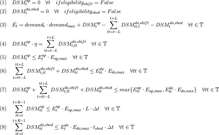
pyomo.core.base.block.SimpleBlockConstraints for SinkDSM with “DLR” approach
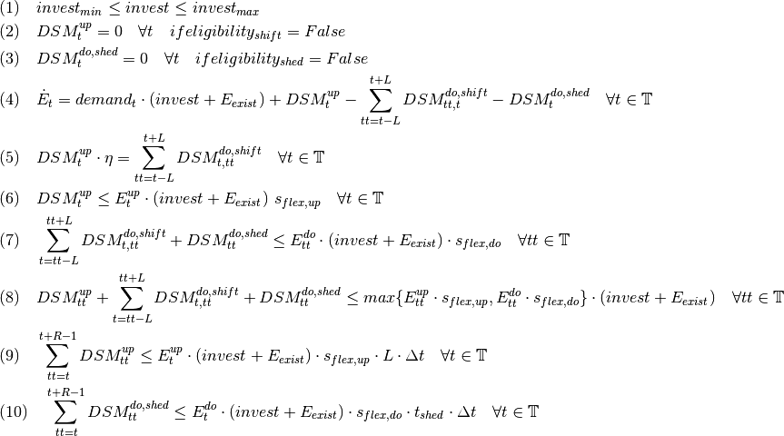
The following constraints are created for approach = ‘DLR’:
![&
(1) \quad DSM_{h, t}^{up} = 0 \quad \forall h \in H_{DR}
\forall t \in \mathbb{T}
\quad if \space eligibility_{shift} = False \\
&
(2) \quad DSM_{t}^{do, shed} = 0 \quad \forall t \in \mathbb{T}
\quad if \space eligibility_{shed} = False \\
&
(3) \quad \dot{E}_{t} = demand_{t} \cdot demand_{max} +
\displaystyle\sum_{h=1}^{H_{DR}} (DSM_{h, t}^{up}
+ DSM_{h, t}^{balanceDo} - DSM_{h, t}^{do, shift}
- DSM_{h, t}^{balanceUp}) - DSM_{t}^{do, shed}
\quad \forall t \in \mathbb{T} \\
&
(4) \quad DSM_{h, t}^{balanceDo} =
\frac{DSM_{h, t - h}^{do, shift}}{\eta}
\quad \forall h \in H_{DR} \forall t \in [h..T] \\
&
(5) \quad DSM_{h, t}^{balanceUp} =
DSM_{h, t-h}^{up} \cdot \eta
\quad \forall h \in H_{DR} \forall t \in [h..T] \\
&
(6) \quad DSM_{h, t}^{do, shift} = 0
\quad \forall h \in H_{DR}
\forall t \in [T - h..T] \\
&
(7) \quad DSM_{h, t}^{up} = 0
\quad \forall h \in H_{DR}
\forall t \in [T - h..T] \\
&
(8) \quad \displaystyle\sum_{h=1}^{H_{DR}} (DSM_{h, t}^{do, shift}
+ DSM_{h, t}^{balanceUp}) + DSM_{t}^{do, shed}
\leq E_{t}^{do} \cdot E_{max, do}
\quad \forall t \in \mathbb{T} \\
&
(9) \quad \displaystyle\sum_{h=1}^{H_{DR}} (DSM_{h, t}^{up}
+ DSM_{h, t}^{balanceDo})
\leq E_{t}^{up} \cdot E_{max, up}
\quad \forall t \in \mathbb{T} \\
&
(10) \quad \Delta t \cdot \displaystyle\sum_{h=1}^{H_{DR}}
(DSM_{h, t}^{do, shift} - DSM_{h, t}^{balanceDo} \cdot \eta)
= W_{t}^{levelDo} - W_{t-1}^{levelDo}
\quad \forall t \in [1..T] \\
&
(11) \quad \Delta t \cdot \displaystyle\sum_{h=1}^{H_{DR}}
(DSM_{h, t}^{up} \cdot \eta - DSM_{h, t}^{balanceUp})
= W_{t}^{levelUp} - W_{t-1}^{levelUp}
\quad \forall t \in [1..T] \\
&
(12) \quad W_{t}^{levelDo} \leq \overline{E}_{t}^{do}
\cdot E_{max, do} \cdot t_{shift}
\quad \forall t \in \mathbb{T} \\
&
(13) \quad W_{t}^{levelUp} \leq \overline{E}_{t}^{up}
\cdot E_{max, up} \cdot t_{shift}
\quad \forall t \in \mathbb{T} \\
&
(14) \quad \displaystyle\sum_{t=0}^{T} DSM_{t}^{do, shed}
\leq E_{max, do} \cdot \overline{E}_{t}^{do} \cdot t_{shed}
\cdot n^{yearLimitShed} \\
&
(15) \quad \displaystyle\sum_{t=0}^{T} \sum_{h=1}^{H_{DR}}
DSM_{h, t}^{do, shift}
\leq E_{max, do} \cdot \overline{E}_{t}^{do} \cdot t_{shift}
\cdot n^{yearLimitShift} \\
(optional \space constraint) \\
&
(16) \quad \displaystyle\sum_{t=0}^{T} \sum_{h=1}^{H_{DR}}
DSM_{h, t}^{up}
\leq E_{max, up} \cdot \overline{E}_{t}^{up} \cdot t_{shift}
\cdot n^{yearLimitShift} \\
(optional \space constraint) \\
&
(17) \quad \displaystyle\sum_{h=1}^{H_{DR}} DSM_{h, t}^{do, shift}
\leq E_{max, do} \cdot \overline{E}_{t}^{do}
\cdot t_{shift} -
\displaystyle\sum_{t'=1}^{t_{dayLimit}} \sum_{h=1}^{H_{DR}}
DSM_{h, t - t'}^{do, shift}
\quad \forall t \in [t-t_{dayLimit}..T] \\
(optional \space constraint) \\
&
(18) \quad \displaystyle\sum_{h=1}^{H_{DR}} DSM_{h, t}^{up}
\leq E_{max, up} \cdot \overline{E}_{t}^{up}
\cdot t_{shift} -
\displaystyle\sum_{t'=1}^{t_{dayLimit}} \sum_{h=1}^{H_{DR}}
DSM_{h, t - t'}^{up}
\quad \forall t \in [t-t_{dayLimit}..T] \\
(optional \space constraint) \\
&
(19) \quad \displaystyle\sum_{h=1}^{H_{DR}} (DSM_{h, t}^{up}
+ DSM_{h, t}^{balanceDo}
+ DSM_{h, t}^{do, shift} + DSM_{h, t}^{balanceUp})
+ DSM_{t}^{do, shed}
\leq \max \{E_{t}^{up} \cdot E_{max, up},
E_{t}^{do} \cdot E_{max, do} \}
\quad \forall t \in \mathbb{T} \\
(optional \space constraint) \\
&](../_images/math/112b3ca10126c08763f355a8d60477cc456dce2b.png)
Note: For the sake of readability, the handling of indices is not displayed here. E.g. evaluating a variable for t-L may lead to a negative and therefore infeasible index. This is addressed by limiting the sums to non-negative indices within the model index bounds. Please refer to the constraints implementation themselves.
The following parts of the objective function are created:

Table: Symbols and attribute names of variables and parameters
Variables (V) and Parameters (P)¶ symbol attribute type explanation 
dsm_up[g,h,t]V DSM up shift (additional load) in hour t with delay time h 
dsm_do_shift[g,h, t]V DSM down shift (less load) in hour t with delay time h 
balance_dsm_up[g,h,t]V DSM down shift (less load) in hour t with delay time h to balance previous upshift 
balance_dsm_do[g,h,t]V DSM up shift (additional load) in hour t with delay time h to balance previous downshift dsm_do_shed[g, t]V DSM shedded (capacity shedded, i.e. not compensated for) flow[g,t]V Energy flowing in from (electrical) inflow bus 
element of delay_timeP delay time for load shift (integer value from set of feasible delay times per DSM portfolio) (time until the energy balance has to be levelled out again; roundtrip time of one load shifting cycle, i.e. time window for upshift and compensating downshift) 
range(length(:attr:`~SinkDSM.delay_time) + 1)` P Set of feasible delay times for load shift of a certain DSM portfolio (time until the energy balance has to be levelled out again; roundtrip time of one load shifting cycle, i.e. time window for upshift and compensating downshift) 
shift_timeP Maximum time for a shift in one direction, i. e. maximum time for an upshift or a downshift in a load shifting cycle shed_timeP Maximum time for one load shedding process demand[t]P (Electrical) demand series (normalized) max_demandP Maximum demand value capacity_down[t]P Capacity allowed for a load adjustment downwards (normalized) (DSM down shift + DSM shedded) capacity_up[t]P Capacity allowed for a shift upwards (normalized) (DSM up shift) max_capacity_downP Maximum capacity allowed for a load adjustment downwards (DSM down shift + DSM shedded) max_capacity_upP Capacity allowed for a shift upwards (normalized) (DSM up shift) efficiencyP Efficiency loss for load shifting processes P Set of time steps P Overall amount of time steps (cardinality) shift_eligibilityP Boolean parameter indicating if unit can be used for load shifting shed_eligibilityP Boolean parameter indicating if unit can be used for load shedding cost_dsm_up[t]P Variable costs for an upwards shift cost_dsm_down_shift[t]P Variable costs for a downwards shift (load shifting) cost_dsm_down_shed[t]P Variable costs for shedding load timeincrementP The time increment of the model 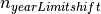
n_yearLimitShiftP Maximum allowed number of load shifts (at full capacity) in the optimization timeframe 
n_yearLimitShedP Maximum allowed number of load sheds (at full capacity) in the optimization timeframe 
t_dayLimitP Maximum duration of load shifts at full capacity per day resp. in the last hours before the current -
CONSTRAINT_GROUP= True
-
-
class
oemof.solph.custom.sink_dsm.SinkDSMDLRInvestmentBlock(*args, **kwargs)[source]¶ Bases:
oemof.solph.custom.sink_dsm.SinkDSMDLRBlockConstraints for SinkDSM with “DLR” approach and
investmentThe following constraints are created for approach = ‘DLR’ with an investment object defined:
![&
(1) \quad invest_{min} \leq invest \leq invest_{max} \\
&
(2) \quad DSM_{h, t}^{up} = 0 \quad \forall h \in H_{DR}
\forall t \in \mathbb{T}
\quad if \space eligibility_{shift} = False \\
&
(3) \quad DSM_{t}^{do, shed} = 0 \quad \forall t \in \mathbb{T}
\quad if \space eligibility_{shed} = False \\
&
(4) \quad \dot{E}_{t} = demand_{t} \cdot (invest + E_{exist})
+ \displaystyle\sum_{h=1}^{H_{DR}} (DSM_{h, t}^{up}
+ DSM_{h, t}^{balanceDo} - DSM_{h, t}^{do, shift}
- DSM_{h, t}^{balanceUp}) - DSM_{t}^{do, shed}
\quad \forall t \in \mathbb{T} \\
&
(5) \quad DSM_{h, t}^{balanceDo} =
\frac{DSM_{h, t - h}^{do, shift}}{\eta}
\quad \forall h \in H_{DR} \forall t \in [h..T] \\
&
(6) \quad DSM_{h, t}^{balanceUp} =
DSM_{h, t-h}^{up} \cdot \eta
\quad \forall h \in H_{DR} \forall t \in [h..T] \\
&
(7) \quad DSM_{h, t}^{do, shift} = 0
\quad \forall h \in H_{DR}
\forall t \in [T - h..T] \\
&
(8) \quad DSM_{h, t}^{up} = 0
\quad \forall h \in H_{DR}
\forall t \in [T - h..T] \\
&
(9) \quad \displaystyle\sum_{h=1}^{H_{DR}} (DSM_{h, t}^{do, shift}
+ DSM_{h, t}^{balanceUp}) + DSM_{t}^{do, shed}
\leq E_{t}^{do} \cdot (invest + E_{exist})
\cdot s_{flex, do}
\quad \forall t \in \mathbb{T} \\
&
(10) \quad \displaystyle\sum_{h=1}^{H_{DR}} (DSM_{h, t}^{up}
+ DSM_{h, t}^{balanceDo})
\leq E_{t}^{up} \cdot (invest + E_{exist})
\cdot s_{flex, up}
\quad \forall t \in \mathbb{T} \\
&
(11) \quad \Delta t \cdot \displaystyle\sum_{h=1}^{H_{DR}}
(DSM_{h, t}^{do, shift} - DSM_{h, t}^{balanceDo} \cdot \eta)
= W_{t}^{levelDo} - W_{t-1}^{levelDo}
\quad \forall t \in [1..T] \\
&
(12) \quad \Delta t \cdot \displaystyle\sum_{h=1}^{H_{DR}}
(DSM_{h, t}^{up} \cdot \eta - DSM_{h, t}^{balanceUp})
= W_{t}^{levelUp} - W_{t-1}^{levelUp}
\quad \forall t \in [1..T] \\
&
(13) \quad W_{t}^{levelDo} \leq \overline{E}_{t}^{do}
\cdot (invest + E_{exist})
\cdot s_{flex, do} \cdot t_{shift}
\quad \forall t \in \mathbb{T} \\
&
(14) \quad W_{t}^{levelUp} \leq \overline{E}_{t}^{up}
\cdot (invest + E_{exist})
\cdot s_{flex, up} \cdot t_{shift}
\quad \forall t \in \mathbb{T} \\
&
(15) \quad \displaystyle\sum_{t=0}^{T} DSM_{t}^{do, shed}
\leq (invest + E_{exist})
\cdot s_{flex, do} \cdot \overline{E}_{t}^{do}
\cdot t_{shed}
\cdot n^{yearLimitShed} \\
&
(16) \quad \displaystyle\sum_{t=0}^{T} \sum_{h=1}^{H_{DR}}
DSM_{h, t}^{do, shift}
\leq (invest + E_{exist})
\cdot s_{flex, do} \cdot \overline{E}_{t}^{do}
\cdot t_{shift}
\cdot n^{yearLimitShift} \\
(optional \space constraint) \\
&
(17) \quad \displaystyle\sum_{t=0}^{T} \sum_{h=1}^{H_{DR}}
DSM_{h, t}^{up}
\leq (invest + E_{exist})
\cdot s_{flex, up} \cdot \overline{E}_{t}^{up}
\cdot t_{shift}
\cdot n^{yearLimitShift} \\
(optional \space constraint) \\
&
(18) \quad \displaystyle\sum_{h=1}^{H_{DR}} DSM_{h, t}^{do, shift}
\leq (invest + E_{exist})
\cdot s_{flex, do} \cdot \overline{E}_{t}^{do}
\cdot t_{shift} -
\displaystyle\sum_{t'=1}^{t_{dayLimit}} \sum_{h=1}^{H_{DR}}
DSM_{h, t - t'}^{do, shift}
\quad \forall t \in [t-t_{dayLimit}..T] \\
(optional \space constraint) \\
&
(19) \quad \displaystyle\sum_{h=1}^{H_{DR}} DSM_{h, t}^{up}
\leq (invest + E_{exist})
\cdot s_{flex, up} \cdot \overline{E}_{t}^{up}
\cdot t_{shift} -
\displaystyle\sum_{t'=1}^{t_{dayLimit}} \sum_{h=1}^{H_{DR}}
DSM_{h, t - t'}^{up}
\quad \forall t \in [t-t_{dayLimit}..T] \\
(optional \space constraint) \\
&
(20) \quad \displaystyle\sum_{h=1}^{H_{DR}} (DSM_{h, t}^{up}
+ DSM_{h, t}^{balanceDo}
+ DSM_{h, t}^{do, shift} + DSM_{h, t}^{balanceUp})
+ DSM_{t}^{shed}
\leq \max \{E_{t}^{up} \cdot s_{flex, up},
E_{t}^{do} \cdot s_{flex, do} \} \cdot (invest + E_{exist})
\quad \forall t \in \mathbb{T} \\
(optional \space constraint) \\
&](../_images/math/144d0ca327bd7c0802d487f66c89ba020f473168.png)
Note: For the sake of readability, the handling of indices is not displayed here. E.g. evaluating a variable for t-L may lead to a negative and therefore infeasible index. This is addressed by limiting the sums to non-negative indices within the model index bounds. Please refer to the constraints implementation themselves.
The following parts of the objective function are created:
- Investment annuity:
- Variable costs:
Table: Symbols and attribute names of variables and parameters
Please refer to
oemof.solph.custom.SinkDSMDLRBlock.The following variables and parameters are exclusively used for investment modeling:
Variables (V) and Parameters (P)¶ symbol attribute type explanation investV DSM capacity invested in. Equals to the additionally installed capacity. The capacity share eligible for a shift is determined by flex share(s). minimumP minimum investment maximumP maximum investment existingP existing DSM capacity flex_share_upP Share of invested capacity that may be shift upwards at maximum flex_share_doP Share of invested capacity that may be shift downwards at maximum ep_costsP specific investment annuity -
CONSTRAINT_GROUP= True
-
class
oemof.solph.custom.sink_dsm.SinkDSMOemofBlock(*args, **kwargs)[source]¶ Bases:
pyomo.core.base.block.SimpleBlockConstraints for SinkDSM with “oemof” approach
The following constraints are created for approach = ‘oemof’:
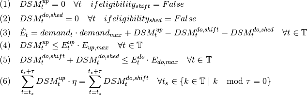
The following parts of the objective function are created:

Table: Symbols and attribute names of variables and parameters
Variables (V) and Parameters (P)¶ symbol attribute type explanation dsm_up[g, t]V DSM up shift (capacity shifted upwards) 
dsm_do_shift[g, t]V DSM down shift (capacity shifted downwards) dsm_do_shed[g, t]V DSM shedded (capacity shedded, i.e. not compensated for) inputsV Energy flowing in from (electrical) inflow bus demand[t]P (Electrical) demand series (normalized) max_demandP Maximum demand value capacity_down[t]P Capacity allowed for a load adjustment downwards (normalized) (DSM down shift + DSM shedded) capacity_up[t]P Capacity allowed for a shift upwards (normalized) (DSM up shift) max_capacity_downP Maximum capacity allowed for a load adjustment downwards (DSM down shift + DSM shedded) max_capacity_upP Capacity allowed for a shift upwards (normalized) (DSM up shift) shift_intervalP Shift interval (time within which the energy balance must be levelled out efficiencyP Efficiency loss forload shifting processes P Time steps shift_eligibilityP Boolean parameter indicating if unit can be used for load shifting shed_eligibilityP Boolean parameter indicating if unit can be used for load shedding cost_dsm_up[t]P Variable costs for an upwards shift cost_dsm_down_shift[t]P Variable costs for a downwards shift (load shifting) cost_dsm_down_shed[t]P Variable costs for shedding load -
CONSTRAINT_GROUP= True
-
-
class
oemof.solph.custom.sink_dsm.SinkDSMOemofInvestmentBlock(*args, **kwargs)[source]¶ Bases:
pyomo.core.base.block.SimpleBlockConstraints for SinkDSM with “oemof” approach and
investmentThe following constraints are created for approach = ‘oemof’ with an investment object defined:
The following parts of the objective function are created:
- Investment annuity:
- Variable costs:

See remarks in
oemof.solph.custom.SinkDSMOemofBlock.Symbols and attribute names of variables and parameters
Please refer to
oemof.solph.custom.SinkDSMOemofBlock.The following variables and parameters are exclusively used for investment modeling:
Variables (V) and Parameters (P)¶ symbol attribute type explanation investV DSM capacity invested in. Equals to the additionally installed capacity. The capacity share eligible for a shift is determined by flex share(s). minimumP minimum investment maximumP maximum investment existingP existing DSM capacity flex_share_upP Share of invested capacity that may be shift upwards at maximum flex_share_doP Share of invested capacity that may be shift downwards at maximum epcostsP specific investment annuity -
CONSTRAINT_GROUP= True
oemof.solph.groupings module
Groupings needed on an energy system for it to work with solph.
If you want to use solph on an energy system, you need to create it with these groupings specified like this:
from oemof.network import EnergySystem import solph
energy_system = EnergySystem(groupings=solph.GROUPINGS)
-
oemof.solph.groupings.constraint_grouping(node, fallback=<function <lambda>>)[source]¶ Grouping function for constraints.
This function can be passed in a list to
groupingsofoemof.solph.network.EnergySystem.Parameters: - node (
Node <oemof.network.Node) – The node for which the figure out a constraint group. - fallback (callable, optional) – A function of one argument. If node doesn’t have a constraint_group attribute, this is used to group the node instead. Defaults to not group the node at all.
- node (
oemof.solph.helpers module
This is a collection of helper functions which work on their own and can be used by various classes. If there are too many helper-functions, they will be sorted in different modules.
-
oemof.solph.helpers.calculate_timeincrement(timeindex, fill_value=None)[source]¶ Calculates timeincrement for timeindex
Parameters: - timeindex (pd.DatetimeIndex) – timeindex of energysystem
- fill_value (numerical) – timeincrement for first timestep in hours
-
oemof.solph.helpers.extend_basic_path(subfolder)[source]¶ Returns a path based on the basic oemof path and creates it if necessary. The subfolder is the name of the path extension.
-
oemof.solph.helpers.flatten(d, parent_key='', sep='_')[source]¶ Flatten dictionary by compressing keys.
- See: https://stackoverflow.com/questions/6027558/
- flatten-nested-python-dictionaries-compressing-keys
d : dictionary sep : separator for flattening keys
Returns: dict
oemof.solph.models module
Solph Optimization Models.
-
class
oemof.solph.models.BaseModel(energysystem, **kwargs)[source]¶ Bases:
pyomo.core.base.PyomoModel.ConcreteModelThe BaseModel for other solph-models (Model, MultiPeriodModel, etc.)
Parameters: - energysystem (EnergySystem object) – Object that holds the nodes of an oemof energy system graph
- constraint_groups (list (optional)) – Solph looks for these groups in the given energy system and uses them to create the constraints of the optimization problem. Defaults to Model.CONSTRAINTS
- objective_weighting (array like (optional)) – Weights used for temporal objective function expressions. If nothing is passed timeincrement will be used which is calculated from the freq length of the energy system timeindex .
- auto_construct (boolean) – If this value is true, the set, variables, constraints, etc. are added, automatically when instantiating the model. For sequential model building process set this value to False and use methods _add_parent_block_sets, _add_parent_block_variables, _add_blocks, _add_objective
- Attributes
- ———–
- timeincrement (sequence) – Time increments.
- flows (dict) – Flows of the model.
- name (str) – Name of the model.
- es (solph.EnergySystem) – Energy system of the model.
- meta (pyomo.opt.results.results_.SolverResults or None) – Solver results.
- dual (… or None)
- rc (… or None)
-
CONSTRAINT_GROUPS= []
-
receive_duals()[source]¶ Method sets solver suffix to extract information about dual variables from solver. Shadow prices (duals) and reduced costs (rc) are set as attributes of the model.
-
solve(solver='cbc', solver_io='lp', **kwargs)[source]¶ Takes care of communication with solver to solve the model.
Parameters: - solver (string) – solver to be used e.g. “glpk”,”gurobi”,”cplex”
- solver_io (string) – pyomo solver interface file format: “lp”,”python”,”nl”, etc.
- **kwargs (keyword arguments) – Possible keys can be set see below:
Other Parameters: - solve_kwargs (dict) – Other arguments for the pyomo.opt.SolverFactory.solve() method Example : {“tee”:True}
- cmdline_options (dict) – Dictionary with command line options for solver e.g. {“mipgap”:”0.01”} results in “–mipgap 0.01” {“interior”:” “} results in “–interior” Gurobi solver takes numeric parameter values such as {“method”: 2}
-
class
oemof.solph.models.Model(energysystem, **kwargs)[source]¶ Bases:
oemof.solph.models.BaseModelAn energy system model for operational and investment optimization.
Parameters: - energysystem (EnergySystem object) – Object that holds the nodes of an oemof energy system graph
- constraint_groups (list) – Solph looks for these groups in the given energy system and uses them to create the constraints of the optimization problem. Defaults to Model.CONSTRAINTS
- **The following basic sets are created**
- NODES – A set with all nodes of the given energy system.
- TIMESTEPS – A set with all timesteps of the given time horizon.
- FLOWS – A 2 dimensional set with all flows. Index: (source, target)
- **The following basic variables are created**
- flow – Flow from source to target indexed by FLOWS, TIMESTEPS. Note: Bounds of this variable are set depending on attributes of the corresponding flow object.
-
CONSTRAINT_GROUPS= [<class 'oemof.solph.blocks.bus.Bus'>, <class 'oemof.solph.blocks.transformer.Transformer'>, <class 'oemof.solph.blocks.investment_flow.InvestmentFlow'>, <class 'oemof.solph.blocks.flow.Flow'>, <class 'oemof.solph.blocks.non_convex_flow.NonConvexFlow'>]
oemof.solph.network module
Classes used to model energy supply systems within solph.
Classes are derived from oemof core network classes and adapted for specific optimization tasks. An energy system is modelled as a graph/network of nodes with very specific constraints on which types of nodes are allowed to be connected.
oemof.solph.options module
Optional classes to be added to a network class.
-
class
oemof.solph.options.Investment(maximum=inf, minimum=0, ep_costs=0, existing=0, nonconvex=False, offset=0, **kwargs)[source]¶ Bases:
objectParameters: - maximum (float, or ) – Maximum of the additional invested capacity
- minimum (float, or ) – Minimum of the additional invested capacity. If nonconvex is True,
minimum defines the threshold for the invested capacity.
- ep_costs (float, ) – Equivalent periodical costs for the investment per flow capacity.
- existing (float, or ) – Existing / installed capacity. The invested capacity is added on top
of this value. Not applicable if nonconvex is set to True.
- nonconvex (bool) – If True, a binary variable for the status of the investment is created. This enables additional fix investment costs (offset) independent of the invested flow capacity. Therefore, use the offset parameter.
- offset (float, ) – Additional fix investment costs. Only applicable if nonconvex is set
to True.
For the variables, constraints and parts of the objective function, which are created, see
oemof.solph.blocks.investment_flow.InvestmentFlowandoemof.solph.components.generic_storage.GenericInvestmentStorageBlock.- maximum (float,
-
class
oemof.solph.options.NonConvex(**kwargs)[source]¶ Bases:
objectParameters: startup_costs (numeric (iterable or scalar)) – Costs associated with a start of the flow (representing a unit).
shutdown_costs (numeric (iterable or scalar)) – Costs associated with the shutdown of the flow (representing a unit).
activity_costs (numeric (iterable or scalar)) – Costs associated with the active operation of the flow, independently from the actual output.
minimum_uptime (numeric (1 or positive integer)) – Minimum time that a flow must be greater then its minimum flow after startup. Be aware that minimum up and downtimes can contradict each other and may lead to infeasible problems.
minimum_downtime (numeric (1 or positive integer)) – Minimum time a flow is forced to zero after shutting down. Be aware that minimum up and downtimes can contradict each other and may to infeasible problems.
maximum_startups (numeric (0 or positive integer)) – Maximum number of start-ups.
maximum_shutdowns (numeric (0 or positive integer)) – Maximum number of shutdowns.
initial_status (numeric (0 or 1)) – Integer value indicating the status of the flow in the first time step (0 = off, 1 = on). For minimum up and downtimes, the initial status is set for the respective values in the edge regions e.g. if a minimum uptime of four timesteps is defined, the initial status is fixed for the four first and last timesteps of the optimization period. If both, up and downtimes are defined, the initial status is set for the maximum of both e.g. for six timesteps if a minimum downtime of six timesteps is defined in addition to a four timestep minimum uptime.
positive_gradient (
dict, default: {‘ub’: None, ‘costs’: 0}) –A dictionary containing the following two keys:
- ‘ub’: numeric (iterable, scalar or None), the normed upper bound on the positive difference (flow[t-1] < flow[t]) of two consecutive flow values.
- ‘costs`: numeric (scalar or None), the gradient cost per unit.
negative_gradient (
dict, default: {‘ub’: None, ‘costs’: 0}) –A dictionary containing the following two keys:
- ‘ub’: numeric (iterable, scalar or None), the normed upper bound on the negative difference (flow[t-1] > flow[t]) of two consecutive flow values.
- ‘costs`: numeric (scalar or None), the gradient cost per unit.
-
max_up_down¶ Compute or return the _max_up_down attribute.
oemof.solph.plumbing module
Plumbing stuff.
-
oemof.solph.plumbing.sequence(iterable_or_scalar)[source]¶ Tests if an object is iterable (except string) or scalar and returns a the original sequence if object is an iterable and a ‘emulated’ sequence object of class _Sequence if object is a scalar or string.
Parameters: iterable_or_scalar (iterable or None or int or float) Examples
>>> sequence([1,2])
[1, 2]
>>> x = sequence(10)
>>> x[0]
10
>>> x[10]
10
>>> print(x)
[10, 10, 10, 10, 10, 10, 10, 10, 10, 10, 10]
oemof.solph.processing module
Modules for providing a convenient data structure for solph results.
Information about the possible usage is provided within the examples.
-
oemof.solph.processing.convert_keys_to_strings(result, keep_none_type=False)[source]¶ Convert the dictionary keys to strings.
All (tuple) keys of the result object e.g. results[(pp1, bus1)] are converted into strings that represent the object labels e.g. results[(‘pp1’,’bus1’)].
-
oemof.solph.processing.create_dataframe(om)[source]¶ Create a result dataframe with all optimization data.
Results from Pyomo are written into pandas DataFrame where separate columns are created for the variable index e.g. for tuples of the flows and components or the timesteps.
-
oemof.solph.processing.get_timestep(x)[source]¶ Get the timestep from oemof tuples.
The timestep from tuples (n, n, int), (n, n), (n, int) and (n,) is fetched as the last element. For time-independent data (scalars) zero ist returned.
-
oemof.solph.processing.get_tuple(x)[source]¶ Get oemof tuple within iterable or create it.
Tuples from Pyomo are of type (n, n, int), (n, n) and (n, int). For single nodes n a tuple with one object (n,) is created.
-
oemof.solph.processing.meta_results(om, undefined=False)[source]¶ Fetch some meta data from the Solver. Feel free to add more keys.
Valid keys of the resulting dictionary are: ‘objective’, ‘problem’, ‘solver’.
- om : oemof.solph.Model
- A solved Model.
- undefined : bool
- By default (False) only defined keys can be found in the dictionary. Set to True to get also the undefined keys.
Returns: dict
-
oemof.solph.processing.parameter_as_dict(system, exclude_none=True, exclude_attrs=None)[source]¶ Create a result dictionary containing node parameters.
Results are written into a dictionary of pandas objects where a Series holds all scalar values and a dataframe all sequences for nodes and flows. The dictionary is keyed by flows (n, n) and nodes (n, None), e.g. parameter[(n, n)][‘sequences’] or parameter[(n, n)][‘scalars’].
Parameters: - system (energy_system.EnergySystem) – A populated energy system.
- exclude_none (bool) – If True, all scalars and sequences containing None values are excluded
- exclude_attrs (Optional[List[str]]) – Optional list of additional attributes which shall be excluded from parameter dict
Returns: dict (Parameters for all nodes and flows)
-
oemof.solph.processing.remove_timestep(x)[source]¶ Remove the timestep from oemof tuples.
The timestep is removed from tuples of type (n, n, int) and (n, int).
-
oemof.solph.processing.results(om)[source]¶ Create a result dictionary from the result DataFrame.
Results from Pyomo are written into a dictionary of pandas objects where a Series holds all scalar values and a dataframe all sequences for nodes and flows. The dictionary is keyed by the nodes e.g. results[idx][‘scalars’] and flows e.g. results[n, n][‘sequences’].
oemof.solph.views module
Modules for providing convenient views for solph results.
Information about the possible usage is provided within the examples.
-
class
oemof.solph.views.NodeOption[source]¶ Bases:
str,enum.EnumAn enumeration.
-
All= 'all'
-
HasInputs= 'has_inputs'
-
HasOnlyInputs= 'has_only_inputs'
-
HasOnlyOutputs= 'has_only_outputs'
-
HasOutputs= 'has_outputs'
-
-
oemof.solph.views.convert_to_multiindex(group, index_names=None, droplevel=None)[source]¶ Convert dict to pandas DataFrame with multiindex
Parameters: - group (dict) – Sequences of the oemof.solph.Model.results dictionary
- index_names (arraylike) – Array with names of the MultiIndex
- droplevel (arraylike) – List containing levels to be dropped from the dataframe
-
oemof.solph.views.filter_nodes(results, option=<NodeOption.All: 'all'>, exclude_busses=False)[source]¶ Get set of nodes from results-dict for given node option.
This function filters nodes from results for special needs. At the moment, the following options are available:
NodeOption.All: ‘all’: Returns all nodesNodeOption.HasOutputs: ‘has_outputs’:- Returns nodes with an output flow (eg. Transformer, Source)
NodeOption.HasInputs: ‘has_inputs’:- Returns nodes with an input flow (eg. Transformer, Sink)
NodeOption.HasOnlyOutputs: ‘has_only_outputs’:- Returns nodes having only output flows (eg. Source)
NodeOption.HasOnlyInputs: ‘has_only_inputs’:- Returns nodes having only input flows (eg. Sink)
Additionally, busses can be excluded by setting exclude_busses to True.
Parameters: - results (dict)
- option (NodeOption)
- exclude_busses (bool) – If set, all bus nodes are excluded from the resulting node set.
Returns: set– A set of Nodes.
-
oemof.solph.views.get_node_by_name(results, *names)[source]¶ Searches results for nodes
Names are looked up in nodes from results and either returned single node (in case only one name is given) or as list of nodes. If name is not found, None is returned.
-
oemof.solph.views.net_storage_flow(results, node_type)[source]¶ Calculates the net storage flow for storage models that have one input edge and one output edge both with flows within the domain of non-negative reals.
Parameters: - results (dict) – A result dictionary from a solved oemof.solph.Model object
- node_type (oemof.solph class) – Specifies the type for which (storage) type net flows are calculated
Returns: - pandas.DataFrame object with multiindex colums. Names of levels of columns
- are (from, to, net_flow.)
Examples
import oemof.solph as solph from oemof.outputlib import views
# solve oemof solph model ‘m’ # Then collect node weights views.net_storage_flow(m.results(), node_type=solph.GenericStorage)
-
oemof.solph.views.node(results, node, multiindex=False, keep_none_type=False)[source]¶ Obtain results for a single node e.g. a Bus or Component.
Either a node or its label string can be passed. Results are written into a dictionary which is keyed by ‘scalars’ and ‘sequences’ holding respective data in a pandas Series and DataFrame.
-
oemof.solph.views.node_input_by_type(results, node_type, droplevel=None)[source]¶ Gets all inputs for all nodes of the type node_type and returns a dataframe.
Parameters: - results (dict) – A result dictionary from a solved oemof.solph.Model object
- node_type (oemof.solph class) – Specifies the type of the node for that inputs are selected
- droplevel (list)
Notes
from oemof import solph from oemof.outputlib import views
# solve oemof solph model ‘m’ # Then collect node weights views.node_input_by_type(m.results(), node_type=solph.Sink)
-
oemof.solph.views.node_output_by_type(results, node_type, droplevel=None)[source]¶ Gets all outputs for all nodes of the type node_type and returns a dataframe.
Parameters: - results (dict) – A result dictionary from a solved oemof.solph.Model object
- node_type (oemof.solph class) – Specifies the type of the node for that outputs are selected
- droplevel (list)
Notes
import oemof.solph as solph from oemof.outputlib import views
# solve oemof solph model ‘m’ # Then collect node weights views.node_output_by_type(m.results(), node_type=solph.Transformer)
-
oemof.solph.views.node_weight_by_type(results, node_type)[source]¶ Extracts node weights (if exist) of all components of the specified node_type.
Node weight are endogenous optimzation variables associated with the node and not the edge between two node, foxample the variable representing the storage level.
Parameters: - results (dict) – A result dictionary from a solved oemof.solph.Model object
- node_type (oemof.solph class) – Specifies the type for which node weights should be collected
Example
from oemof.outputlib import views
# solve oemof model ‘m’ # Then collect node weights views.node_weight_by_type(m.results(), node_type=solph.GenericStorage)